Welcome to Excel Avon
Winner trophy chart in Excel
DOWNLOAD THE USED EXCEL FILE FROM HERE>>
In today’s post we will tell you how to create winner trophy chart in excel yes it may be little different here we will use picture and also use 2-d clustered chart it is very simple yes excel winner trophy The chart looks like a bar chart. The winner trophy chart will give you a very professional feel. This chart, although not commonly used, seems to be Winner’s Trophy is a graph that shows vertical bars with the bar’s axis value displayed on the left side of the graph. Technically, the cloistered chart and online image insert will be used to create the winner’s trophy.
In this article, I will teach you to create winner trophy chart in Excel step by step with pictures.
Well, as you can see, our winner trophy chart is going to be like this.
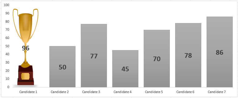
Create Winner trophy chart in Excel
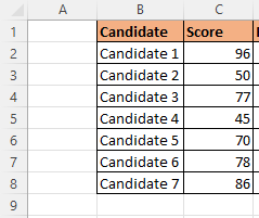
Create a table in excel sheet which will look something like this. In which there will be 2 columns. candidate and score.
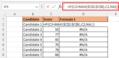
Now insert a new column, write column name formula 1 and then add formula in cell =IF (C8=MAX ($C$2: $C$8),C8,NA()), if the maximum value of score is equal to C2 range up to c2 value will be printed in D2. else if the condition is false N/A. After adding the formula, drag the formula across the column.
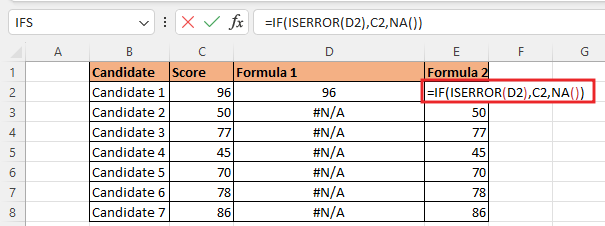
Now insert one more column, write column name formula 2 and then add formula in cell =IF(ISERROR(D2),C2,NA()) if the maximum value of D2 is error then the value condition of C2 is true, Otherwise NA else if the condition is false N/A. After adding the formula, drag the formula across the column. Use format painter to paste the cell’s formatting into another cell.
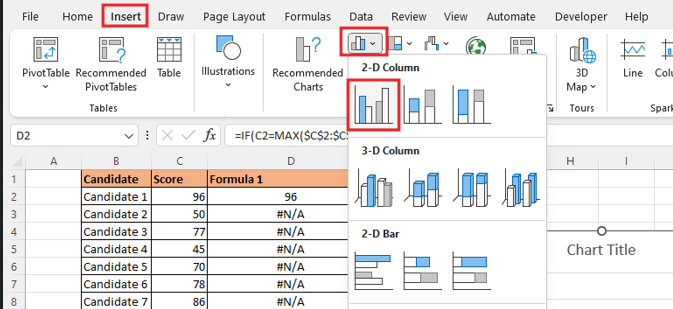
Select Formula 1 and Formula 2 then you go to 2-D Column and insert clustered chart.
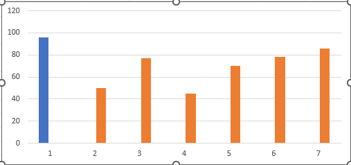
Delete chart title and legend after inserting the chart.
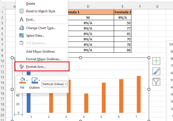
By right click on the Axis, go to the format axis data option.
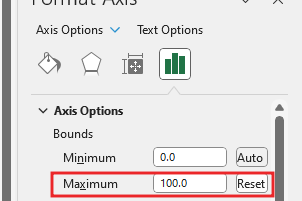
Set the making value of bound to 100 in axis option. This will give your axis a range of 0-100.
Now select the column and now you increase the overlap value of each axis. it reduces that column gap width.
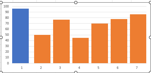
Now right click on select data option. By editing series 1.
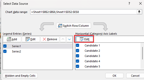
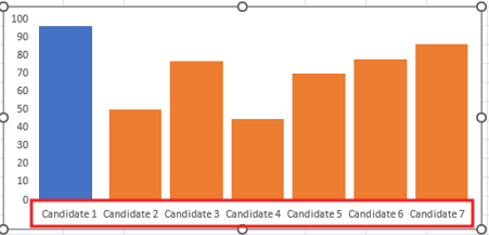
we add candidate column in axis level range.

By adding the candidate column to the data label, we can see the label of all the candidates below the column.
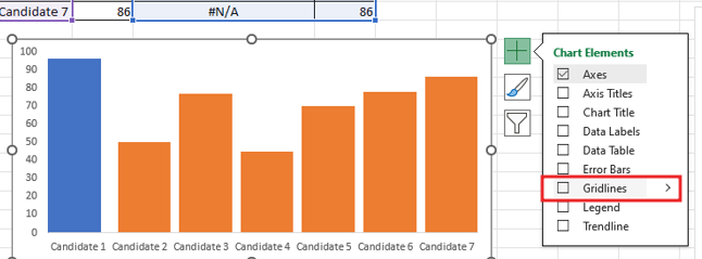
Go to element option and remove gridline from chart.
Now we’ll insert a picture by going to insert tab> illustrations> picture> Online Picture. We are inserting picture online here but if you want to add picture from device then you can go to this device option.
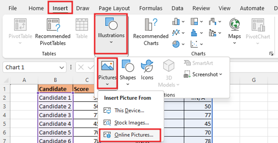
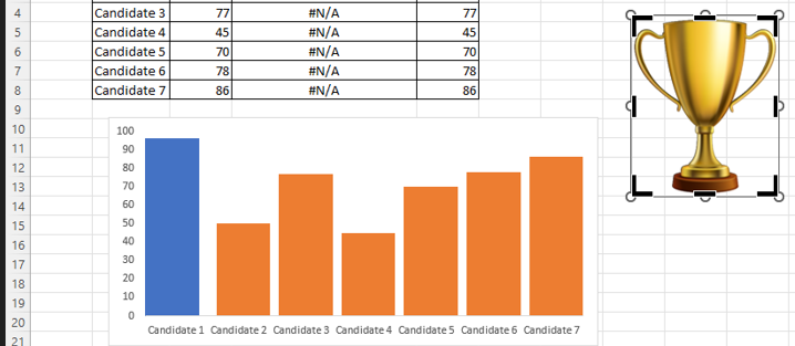
You insert the picture of trophy in the search bar, select a picture of trophy. click insert button then picture will be insert.

After inserting the picture, we will go to picture format tab then select the crop option then cut the trophy picture.
After cropping the picture, you can also use the shortcut to cut it by right click.
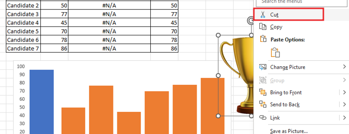
And you paste it in the top value bars as you can see, we have pasted the winner trophy in the blue bars. To fit the picture, drag the chart so that the picture will be perfect in the chart.

Now go to the element option and add the data label and also align the label to the center.

Now we’ll formatting text of the labels, like increase font size then bold and you do more.
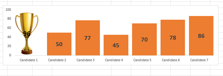
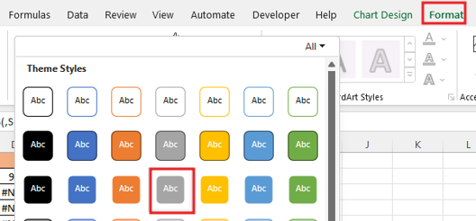
You can make some changes according to yourself like changing the style of bars by going to format option.
Now our chart is ready you can see it something like this our winner trophy chart.

Therefore, I hope that you have understood How to Create winner trophy chart in Excel, maybe if you do not understand anything, then you can comment us with the question, which we will answer soon and for more information, you can follow us on Twitter, Instagram, LinkedIn and you can also follow on YouTube.
DOWNLOAD THE USED EXCEL FILE FROM HERE>>
LEARN MORE DASHBORAD AND CHART TOPIC HERE
You can also see well-explained video here about How to Create winner trophy Chart in Excel


