Welcome to Excel Avon
Waffle chart with the conditional formatting in Excel
DOWNLOAD THE USED EXCEL FROM HERE>>
In today’s post we will explain How to Create Waffle chart with the conditional formatting in excel, Excel waffle charts are a popular way to display parts of a whole. Waffle chart grabs readers attention and can effectively be to used to highlight a specific meter, you can think of these as an alternative to pie and donut charts. We’ll start with a waffle chart that adds up to 100% using a 10 x 10 grid of cells, also known as relative waffle charts.
So today in this article, I will explain How to Create Waffle chart with the conditional formatting in excel step by step with pictures.

Create Waffle chart with the conditional formatting in Excel
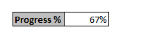
Create a cell in the Excel sheet where the data contains the displayed value, or we can use it as a display cell which will look like this. No formula has been added here. just a simple value.
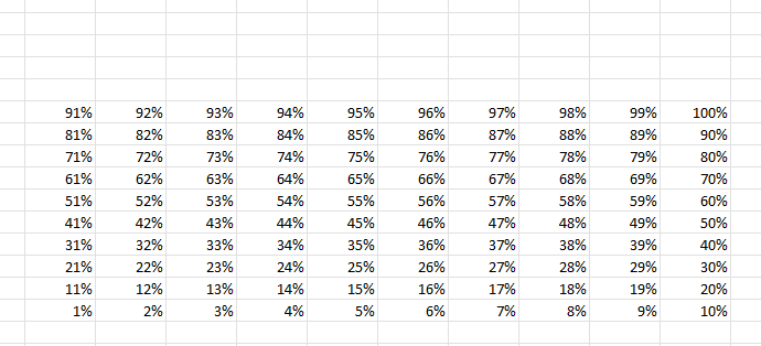
Now you have to write the values which will range from 1 -100 and as we said above, it adds up to 100% using a grid of 10 x 10 cells. Our data will be something like this.
Now select the data you have written and then go to the format option.
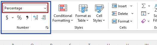
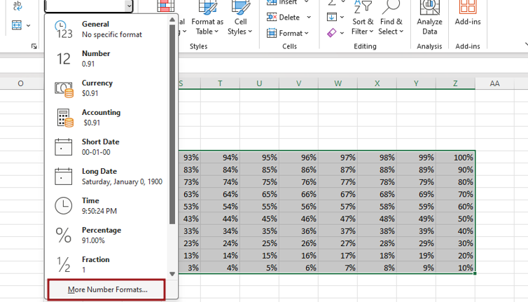
In the No. Format option go to more No. Format option.
After going to More Number format option, you have to select custom option. In custom, you have to write the type as per your choice. As we have used semi colon 3 times in the type, I will explain the reason for using it later.
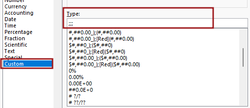
The reason for using semicolon is that changing the data type will make the cell appear blank but the value in the cell will remain the same.

Now select the data again and go to the conditional formatting option, in conditional formatting you will have many options, select the manage rule.
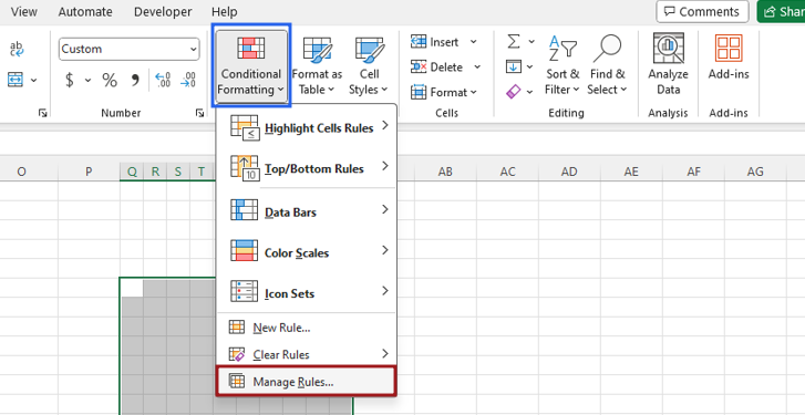
In Manage Rule you will get an option to add, click on Add button.

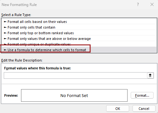
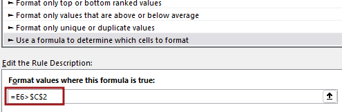
Here you have to add a new rule but there are some rule types also so we will select a rule type and use formula to determine which cells to format.
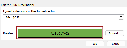
Now you get the option new formatting rule, then we’ll add rule, the value of F6 would be less than of equal to C2(Display Cell) =E6<=$C$2
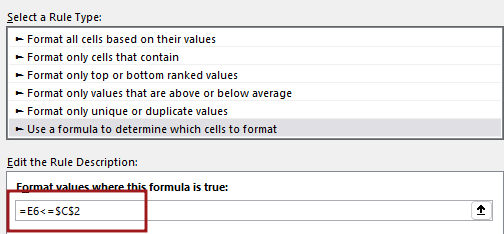
Color formatting will be done for any cell whose value satisfies the above rule. Add color, Then Border style , border color, outline in cell Format.
Once the rule is added, click on the New Rule button again and select the same rule, use formula to determine which cells to format.
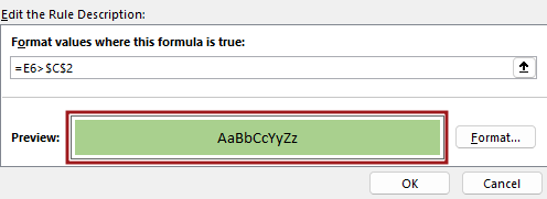
Now the rule will be added when the value F6 is greater than C2(Display Cell) =F6>$C$2
When value satisfied this rule, then color of cell will be like this, Do different formatting from the previous rule formatting. For the first condition dark color was selected, in this rule we are selecting light color.
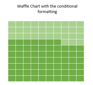
Return to data sheet after applying formatting. As you can see the formatting has been added, as you know we added two rules. the values in the table that satisfy the first rule are filled with dark color and the values that satisfy the Second rule are filled with Light color.
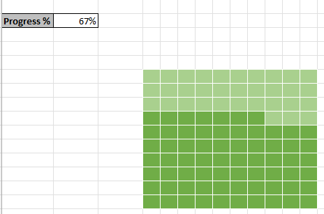
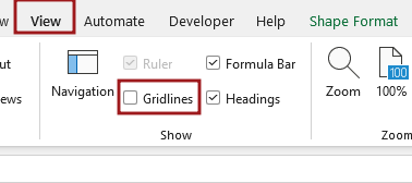
Go to View tab and remove gridline from sheet.
Now we’ll insert a text box by going to Insert tab, after selecting text box drag it in sheet. We also filled the title of the chart.
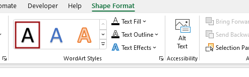
Make Text Box No outline by going to shape format. add style in title text by going wordart style.
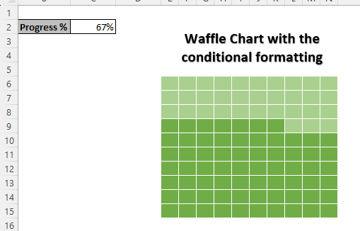
Add finally we have to adjust the text of textbox, aligning bold color, size of font.
Therefore, I hope that you have understood How to Create Waffle chart with the conditional formatting in excel, maybe if you do not understand anything, then you can comment us with the question, which we will answer soon and for more information, you can follow us on Twitter, Instagram, LinkedIn and you can also follow on YouTube.
DOWNLOAD THE USED EXCEL FROM HERE>>
LEARN MORE DASHBORAD AND CHART TOPIC HERE
You can also see well-explained video here about How to Create Waffle chart with the conditional formatting in excel


