Welcome to Excel Avon
Introduction of MATCH Formula
Summary
In this video I will explain How to use MATCH Formula in excel. The MATCH function in Excel searches for a specified value in a range of cells, and returns the relative position of that value.
Formula
=MATCH(lookup_value, lookup_array, [match_type])
Arguments
Lookup_value –the value you are searching for. It can be either numeric, text or logical value as well as a cell reference.lookup_arraylookup_array
Lookup_array – A range of cells or the range of cells to search in.
Match_type – [optional] 0 = exact match, -1 = exact or next largest, 1 = exact or next smallest (default).
The match function is applied only in single column or row and not in multiple column multiple row.
MATCH Formula in Excel
Use in Column
Example 1
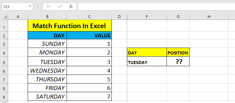
We have made an example to use the match formula. I will use the match formula in column in the first instance. As you can see, in the first image we have some data. We will find value by using the match formula. Use in Column
No I Will Apply Formula.
=MATCH(F5,B3:B9,0) for exact value Zero.
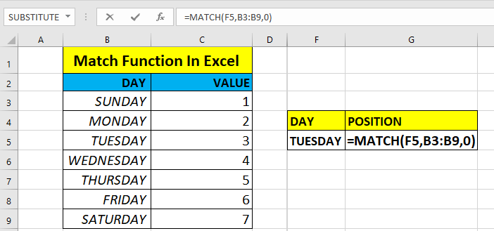
As you can see, we have applied the formula and will find the value of the Tuesday.
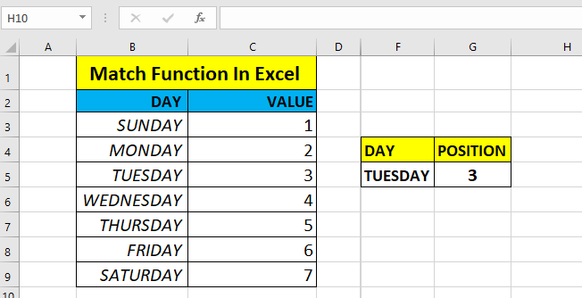
So now using the match formula, the value of the Tuesday has been found.
Use in Row
Now I will use this formula in Row,
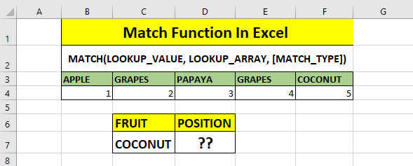
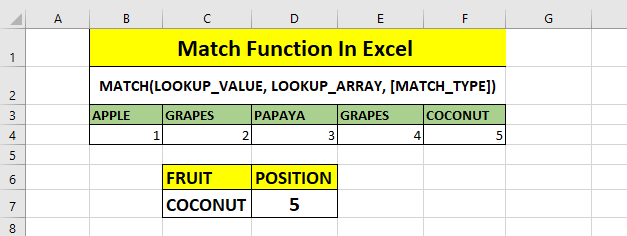
As you can see, the example have been created whose positions will find. formula =MATCH(C7,B3:F3,0)
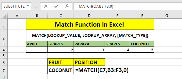
Now I will press enter and we found the position of the coconut (according above image)
-
- In case of duplicates, MATCH returns the first match.
- MATCH is not case-sensitive.
- MATCH only works with text up to 255 characters in length.
So I hope you have understood this formula and for more information you can follow us on Twitter, Instagram, LinkedIn and YouTube as well.


