Welcome to Excel Avon
Insert Slicer in Excel
Slicer is a type of tool which is used in Excel to filter the data as per our requirement by cutting a portion of the data from the table created using the Pivot Table option. First we will create a pivot table as a table to connect the slicers. Which is available under the Insert menu option. Then, in the same Insert menu tab, choose Slicer, which is available under the Filters section. In the Slicer Connection box, we will be able to see an Insert Slicer box with all the available data headers used to create that pivot chart. Now, if we select one or more regions, we will be able to get a slicer box on the screen. Click on any data to filter the table.
How to Insert Slicer in Excel
DOWNLOAD USED EXCEL FILE FROM HERE>>
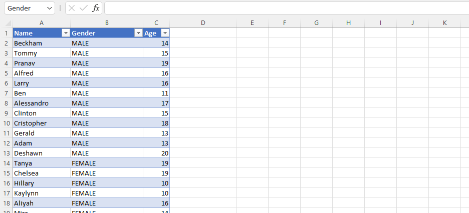
Now let’s understand by example, We have age and gender data for some students as shown below,
We will see how the slicers can be added for this data. You will follow the steps given below.
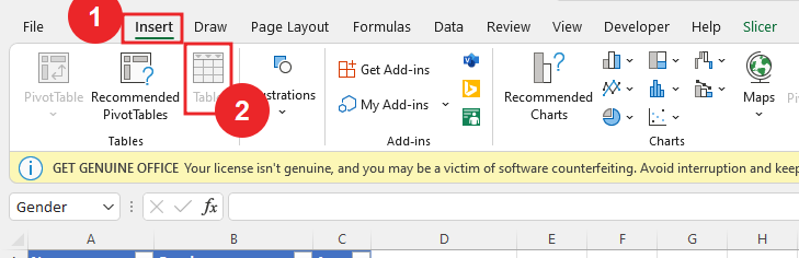
Now we will select the complete data and insert a table which will open a new pop up window named CREATE TABLE in which your selected data will be filled and we will press ok.

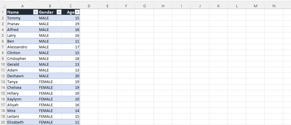
After inserting the table, the table will look like this, you can see Below
When you’ve inserted a table into the data, you’ll see a new tool added to the right side of the upper ribbon pane under the Table Tools option called Table Design.

Go into the Table Design tab, and you’ll see a range of options available under it. Under the Tools section, under the Table Design tab, click the Insert Slicer button. This will allow you to put slicers on the table. You click on the Insert Slicer button under Tools Options under the Design tab, you will see an Insert Slicer window. Inside it, you can have all the columns in the table and use any of them as a slicer.

I’ll choose Age and Gender as slicer options and see what happens. After selecting Age and Gender as the slicers, click on the OK. You can see a slicer added to the bottom of your Excel table with labels for all ages and genders.

You can first use the Age button to filter the data. For example, if I want to see all the data for a 10 year old, both male and female, all I need to do is click the 10-year slicer button and then view. How do we get the result, see the screenshot below.

Once again we can see by using Gender button.

Here we want to extract the mail data of 18 to 20 years. Filter button given in the slicer button will do when we need the data of all the options of that slicer.
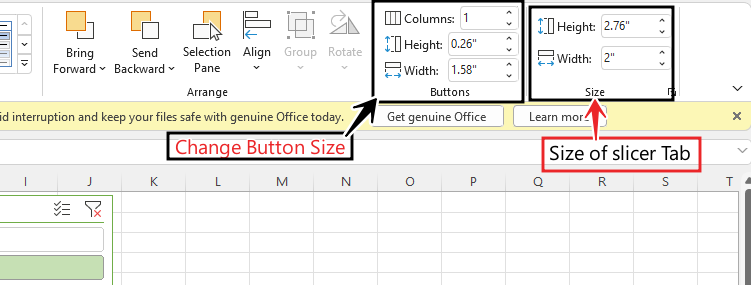
You can Change Slicer Styles here

In the image, we can see how we can change the size of the button and slicer tab, apart from this you can also change the size with the cursor.
- You can change the name of the tab by going to the slicer settings.
- Slicers are nothing more than dynamic filters, which can be applied on Tables, Pivots or Pivot Charts.
DOWNLOAD USED EXCEL FILE FROM HERE>>
So I hope you have understood How to Insert Slicer in Excel and for more information, you can follow us on Twitter, Instagram, LinkedIn, and YouTube as well.
You can also see well-explained video here


")