Welcome to Excel Avon
Use of INDEX and MATCH with multiple criteria
In this Post We will explain How to use INDEX and MATCH with multiple criteria. Using the Index Formula You can use INDEX to retrieve individual values, or entire rows and columns. and The MATCH function in Excel searches for a specified value in a range of cells, and returns the relative position of that value. Index match with multiple criteria enables you to perform a successful lookup when more than one lookup value is matched.
Formula
{=INDEX(Result_Range, MATCH(1, (Criteria1=Criteria1_Range)*(Criteria2=Criteria2_Range)*(Criteria3=Criteria3_Range)...,0))}
Arguments
Result_Range – From which range need to get result based on match.
Criteria1 – Criteria1 Value
Criteria1_Range – Criteria Range for Criteria1.
Criteria2 – Criteria2 Value
Criteria2_Range – Criteria Range for Criteria2
Criteria3 – Criteria3 Value
Criteria3_Range – Criteria Range for Criteria3
(..….) – More Criteria with Criteria Ranges.
INDEX and MATCH with multiple criteria
Download excel file from here>>
As you guys can see we have created a data sheet in which 4 columns are product category, product size, product color and product price.
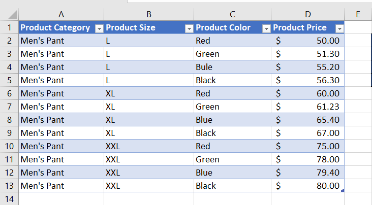
Now suppose to find the price of a product from this sheet with multiple criteria then we have to make the criteria.
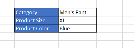
So this is the criteria and we will know the price of the product.
=INDEX(Table1[Product Price],MATCH(1,(G2=Table1[Product Category])*(G3=Table1[Product Size])*(G4=Table1[Product Color]),0))
In Excel-language, 1 means TRUE. 0 means FALSE.
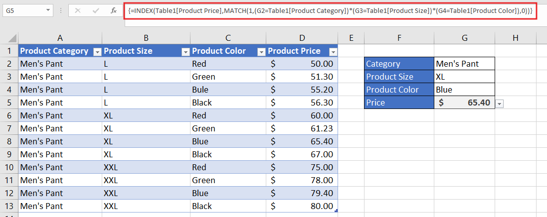
You can see the formula used in the image, we have red marked the formula. do not press Enter when you’re done with the formula. It won’t work. Instead, press and hold Ctrl and Shift and then press Enter. and now you can get the price, based on selected category, size and color.
Note
Combining the Excel INDEX and MATCH function can be more powerful than the VLOOKUP formula.
The MATCH function can return the row number and column number of the table headers of both rows and columns.
Download excel file from here>>
By this way I have clearly explained INDEX and MATCH with multiple criteria
So I hope you have understood this formula and for more information you can follow us on Twitter, Instagram, LinkedIn and YouTube as well.
You can also see well explained video here

