Welcome to Excel Avon
Use IFS Formula in Excel
The IFS function is very easy to use. The IFS function checks whether one or more conditions are observed and returns a value that satisfies the first TRUE condition. Use the IFS function to evaluate multiple conditions without multiple nested. You can use the IFS function when you want a self-contained formula to test multiple conditions at the same time without nesting multiple IF statements. IFS Pay based formulas are shorter and easier to read and write.
Formula
= IFS(test1, Value1 [test2, Value2] ….......
Arguments
Test1 – First logical test. This is a required argument.
Value1 – Result when logical_test1 is true. If necessary, you can leave it blank.
Test 2 – This is an optional parameter that specifies the second test condition, which the function evaluates when the first condition turns out to be FALSE.
Value2 – This is also an optional parameter that specifies the value that is returned if the first condition turns out to be FALSE and the second condition turns out to be TRUE.
How to Use IFS Formula
DOWNLOAD USED EXCEL FILE FROM HERE>>
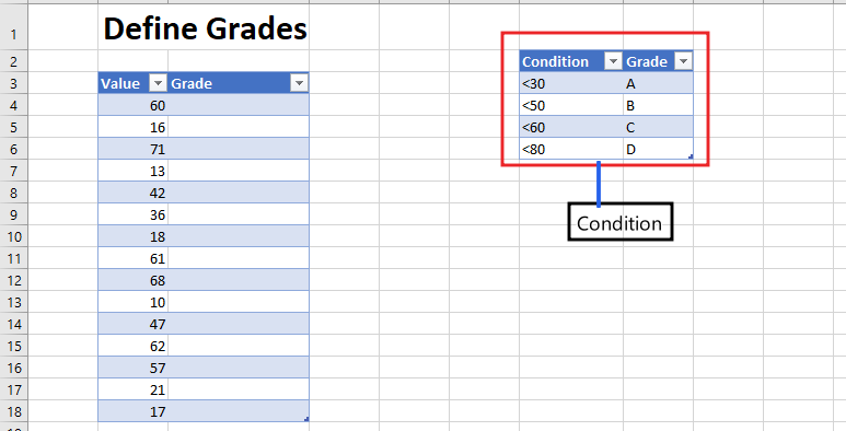
Example 1
As you can see we are given some value in which we will create some condition and apply IFS formula. Separate sheet has been made for the condition. In the first example we can see that we have to define grade condition is if value is 30 or less than 30 then grade is a, if value is 50 or less than 50 then b is if 60 or less than 60 then grade c and if value. 80 or younger than 80 will go to grade D
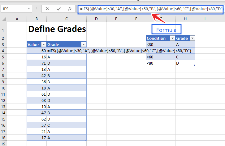
Now we will find the grade of all the given value and apply the IFS formula.
=IFS([@Value]<30,"A",[@Value]<50,"B",[@Value]<60,"C",[@Value]<80,"D")
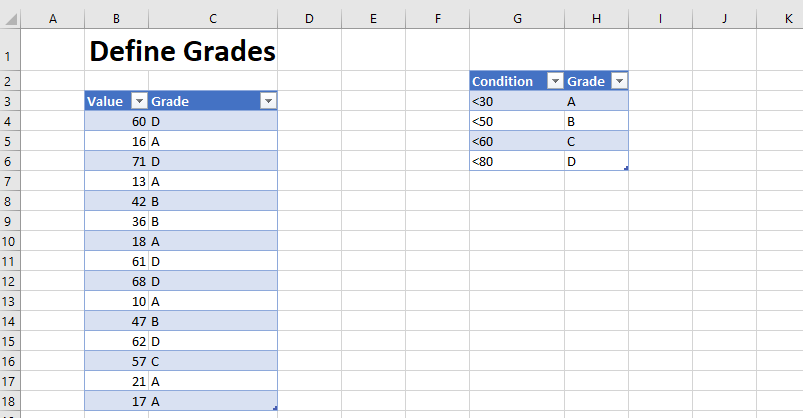
And after applying the formula, we will get everyone’s grades.
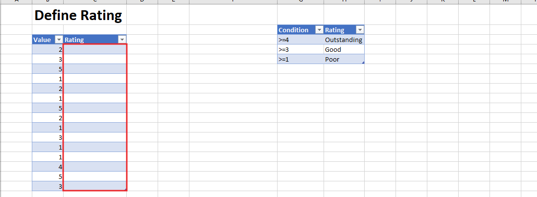
Example 2
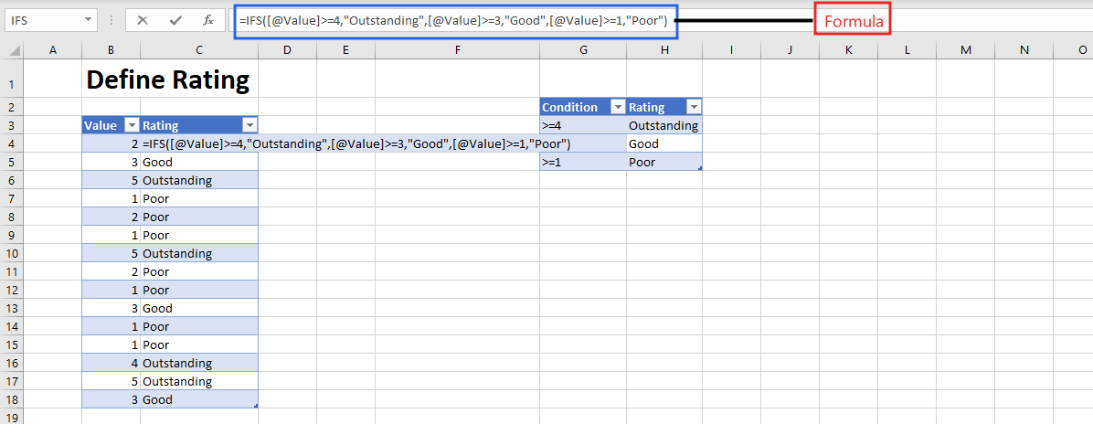
Yes, in example 2 we are going to make condition from value and make rating from condition and apply formula and find rating of all values. In 2nd example you can say we have been given 3 condition, if value is 4 or greater than 4 then outstanding, if value is 3 or 3 then value is good and if value is greater than 1 or 1 then we will get poor rating.
Now we will find the rating of all the given value and apply the IFS formula.
=IFS([@Value]>=4,"Outstanding",[@Value]>=3,"Good",[@Value]>=1,"Poor")
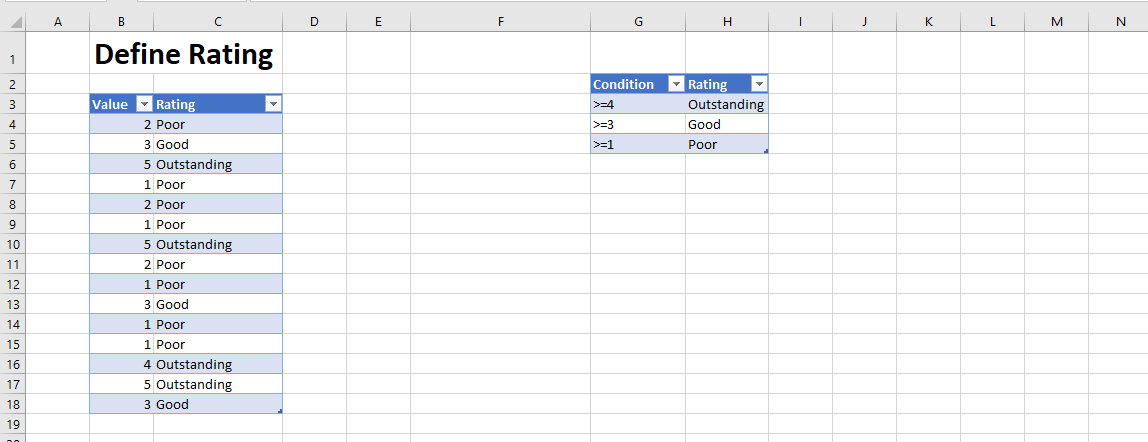
You can see that we have found the rating of the value by applying the IFS formula.
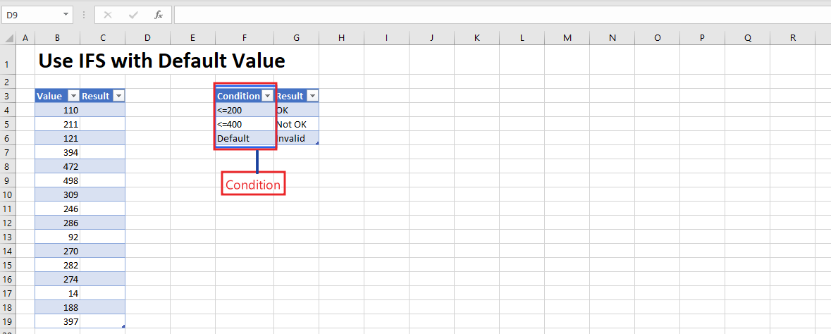
Example 3
In the third example, you can see that we have been given the condition that if the value column has a value of 200 or less than 200, then the result will be OK. And if the value is less than 400 or less than 400 then the result is not ok, and any such value will come which is default then its result will be invalid.
And now we will apply the IFS formula and see the result of all the values.
=IFS([@Value]<=200,"OK",[@Value]<=400,"Not OK",TRUE,"Invalid")
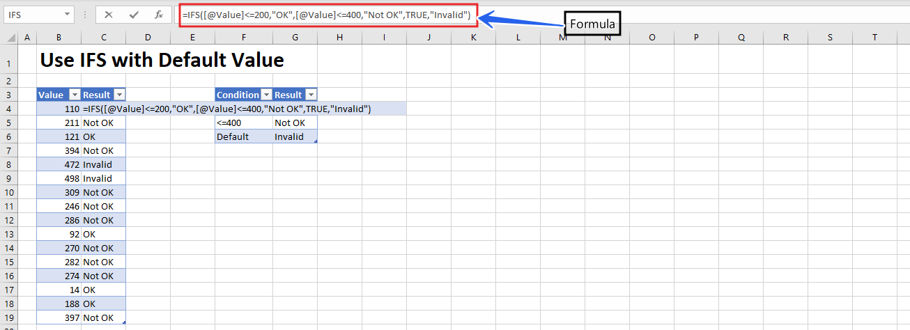
After applying the formula, we have found the result of all the values as can be seen in the given image.
DOWNLOAD USED EXCEL FILE FROM HERE>>
So I hope you have understood this formula and for more information, you can follow us on Twitter, Instagram, LinkedIn, and YouTube as well.
You can also see well-explained video here
")

