Welcome to Excel Avon
Hi guy today I will show you how to use SUMIFS formula in Excel.
Summary
SUMIFS is a function to sum sale that meet multiple criteria. SUMIFS can be used to sum value
when corresponding cells meet criteria based on number, date and text.
Syntax of formula
=SUMIFS(SUM_Range,Range1, Criteria,[Range2],[Criteria2],………)
Arguments
SUM_RANGE -The range to be summed
Range 1 -The range first evaluate.
Criteria -Criteria to use Range1.
Range 2 -The second range to evaluate.
Criteria 2 – The criteria to use Range2
Examples : 1
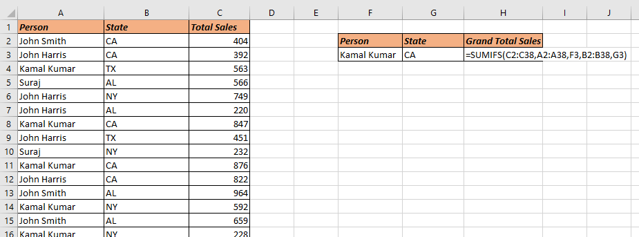
In 1st Example I will use for data base person with state & total sale so I will calculate with two criteria person & state, I will apply formula in here
=SUMIFS(C2:C38,A2:A38,F3,B2:B38,G3)
Where-
C2:C38 is the Range of sum
A2:A38 is the first Range Evaluate
F3 is the criteria
B2:B38 Range2
Now by this you can get the SUM per state the total sale , total sales based on KAMAL KUMAR , KAMAL KUMAR on based CA. According attached below image-

Example:2
In second example of SUMIFS so if I have made the data base with date & sale person & total sales I want to calculate the total sale of person b/w two date so I will use SUMIFS formula with three Criteria I will write here
=SUMIFS(C2:C38,A2:A38,”>=” & F3,A2:A38,”<=” & G3″,B2:B38,H3)
Where-
C2:C38 Is The range to be sum
A2:A38 is the range first evaluate
“>=” & F3 : first criteria
A2:A38 : The second range to evaluate
“<=” & G3 : Second criteria
B2:B38 : The third range to evaluate
H3 : Third criteria
So by this way I have three criteria in this formula and i have used the numeric date with equal or greater and less or equal.
(according attached below image)

You can also see well explained video here


