Welcome to Excel Avon
How to use OFFSET Formula in Excel
SUMMARY
In this post I will Show you how to use OFFSET formula in excel The OFFSET function helps to get the value stored in a selected row or column or array of a row-column matrix by calling out the row and column number with reference to cell value. The OFFSET function starts counting the row and column number once we fix the reference cell and that cells will become its first point to start counting.
FORMULA
ARGUMENTS
Reference- It is the argument from which we want to base the offset. It could be a cell reference or a range of adjacent cell.
Rows – The number of rows to offset below the starting reference.
Column – The number of columns left or right to the starting reference value. This parameter can accept positive or negative values.
Optional Arguments
Height – This argument is optional. It should be a positive number. It is a number that represents the number of rows in the returned reference.
Width – This argument is optional. It should be a positive number. It is a number that represents the number of rows in the returned reference.
Usage Note
-
- OFFSET only returns a reference, no cells are moved.
- Excel documentation says height and width can’t be negative, but negative values do work.
- When height or width is omitted, the height and width of reference is used.
How to use OFFSET Formula in Excel
OFFSET Function in Excel is very simple and easy to use. Let understand the working of the OFFSET Function in Excel by some OFFSET Formula example. As we have made some Example to use the offset formula.

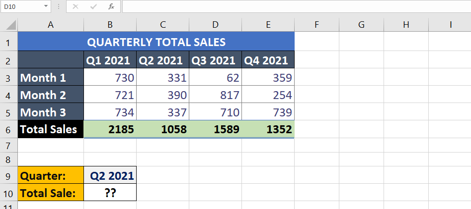
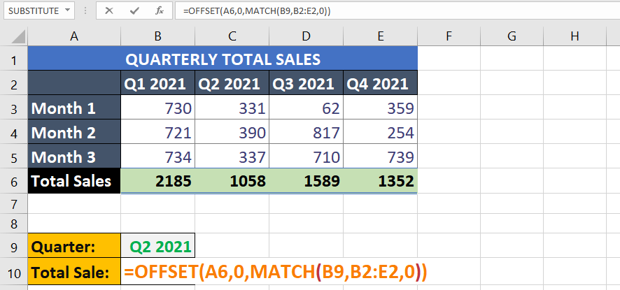
Find out the total sales from the given sales report. So now we will use the formula.
=OFFSET(A6,0,MATCH(B9,B2:E2,0))

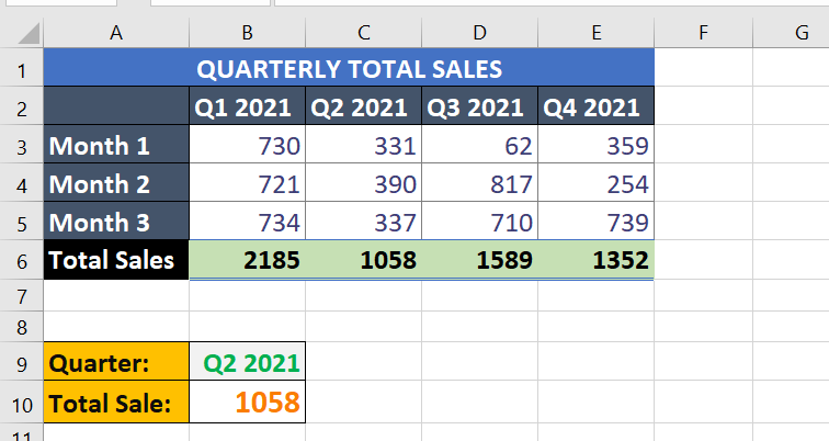
After the formula, I will Press enter for result . Now we know the total sales of Q2 2021.

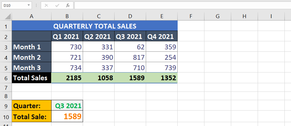
To find out the sales of Q3, To find the Total sales of Q3, we will write Q3 2021 in B9.

You can also check my well explained video about DATEDIF formula


