Welcome to Excel Avon
INDEX MATCH Formula in Excel
The use of INDEX and MATCH formula is very famous formula in excel. This is because the index and match formula is flexible. We can use formula in many places like H-lookups, V-lookups, 2-way lookups, left lookups, case-sensitive lookups, and lookups based multiple criteria. If you want to be pro in excel then you must have knowledge of index and match function.
Summary
These are two different formulas but for now we will do that together.
MATCH Function
The MATCH function in Excel searches for a specified value in a range of cells, and returns the relative position of that value.
=MATCH(lookup_value, lookup_array, [match_type])
INDEX Function
You can use INDEX to retrieve individual values, or entire rows and columns. The MATCH function is often used together with INDEX to provide row and column numbers.
=INDEX (array, row_num, [col_num], [area_num])
Example 1
as you can see I have created some example first column has data of person and second column is salary data now use with index match formula for finding salary of any person.
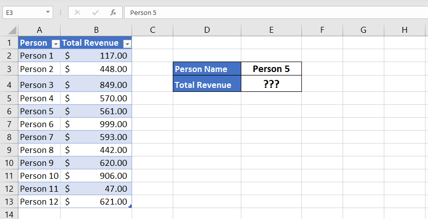
NOW APPLY THE FORMULA.
=INDEX(B2:B13, MATCH(E3, A2, A13,0))
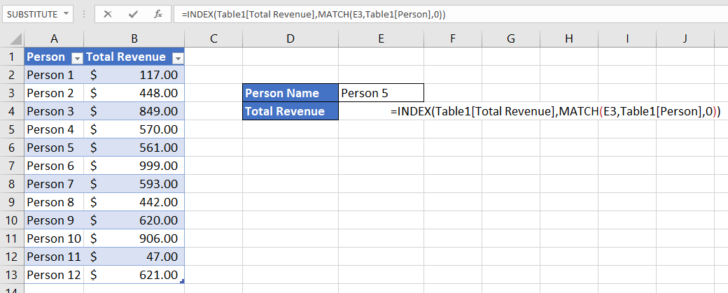
After applying the formula, we will press enter and the salary of Person 5 will be known.
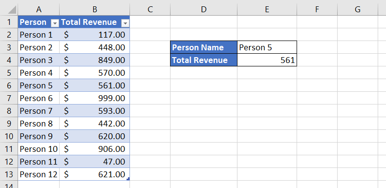
As can be seen in image 3 the salary of Person 5 has been known.
How to use INDEX & MATCH Formula in Excel
Formula 2
As you can see that we have created another sheet for the sample, now we will use the INDEX MATCH formula. In these sheets there are 12 persons and 12 months, in which there is data of salary of every month, so now from this data we will find the salary of 7th person in July.
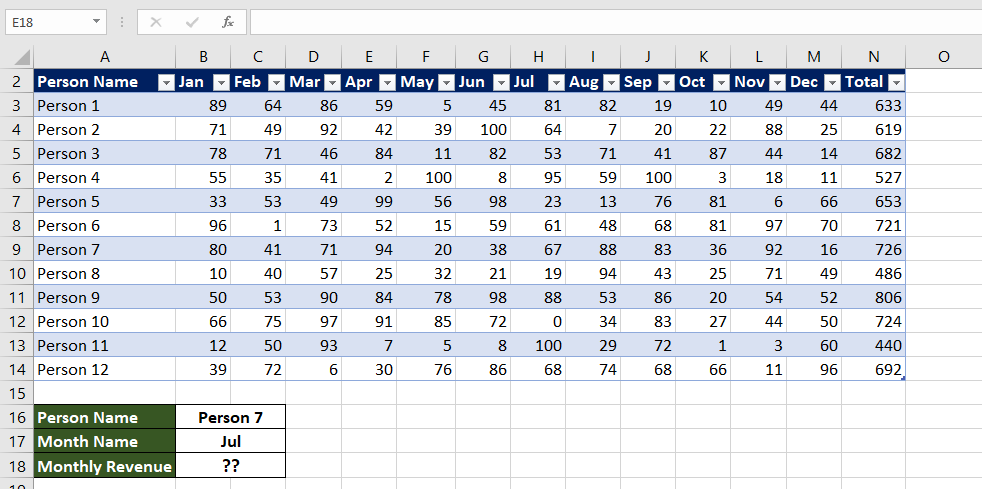
So now we will apply the formula and find out the monthly salary of person 7.
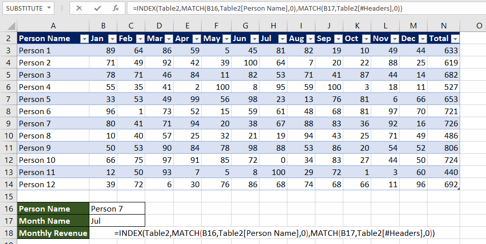
After applying the formula,
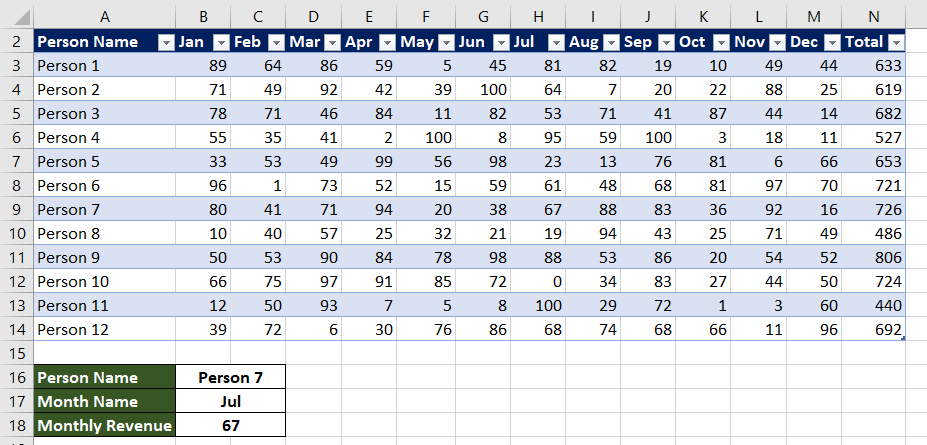
We got to know the monthly salary of Person 7. So I hope you have understood this formula.
You can also check my well explained video about DATEDIF formula


