Welcome to Excel Avon
How To Use INDEX formula in Excel
Summary
In this post I will learn you how to use INDEX formula You can use INDEX to retrieve individual values, or entire rows and columns. The MATCH function is often used together with INDEX to provide row and column numbers.
Formula
Arguments
row_num – The row position in the reference or array.
area_num – [optional] The range in reference that should be used.
How To Use INDEX formula in Excel
Example 1
So friends, In this post, I am to teach you how to use index formula. Index formula is very useful and easy formula. To use index formula we have created some example which is electronic shop data and in that we will find product’s code and rate with index function.

As you can see that we have created a sheet for the sample, now we will use the sample to find the rate of the product.
=Index(B3:F9,3,4)
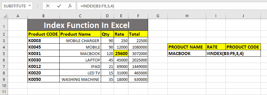
As you can see we have selected array from B3 to F9 and instead of row we have written 3 and in column 4 this is to find the rate of MacBook. After typing the formula, press enter, you will get the rate of MacBook.

The rate of MacBook is 25600 which we have found using index formula.
Example 2
In second example we will find product code by using INDEX formula which is left side of product in excel sheet. so in this also I have to write INDEX formula.
=INDEX(B3:F9,3,1)
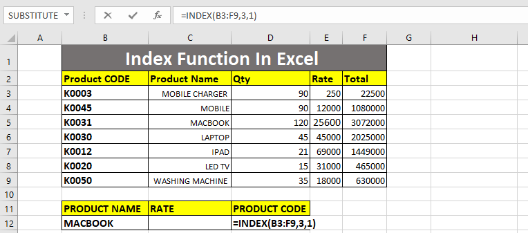
After using the INDEX formula, we will press enter so that we will know the code of the product.
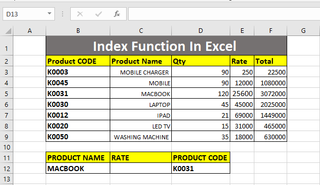
So I hope you have understood this formula.


