Welcome to Excel Avon
What is AGGREGATE Formula
The Excel aggregate function returns the result of a specified operation or function, applied to a list or database of values. The aggregate function includes a number of mathematical functions such as mean, maximum, average, sum, minimum, etc., along with conditions that are optimized for each of these sub-functions available under the aggregate function. We can also ignore different cells or rows like blank row, error value etc and get the output as we want. A total of 19 sub-functions with different options are available in aggregate function.
Formula
=AGGREGATE(function_num,options,array,[k])
Arguments
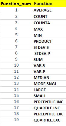
Function_num : This number represents a specific function that is to be used. It ranges from 1-19.
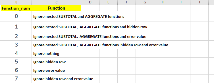
Options : This is a numeric value ranging from 0 to 7. It determines the values that are ignored during calculations.
array : An array or refers to a range of cells when using the ARRAY syntax.
[k]: The last 6 functions (under 1 to 19 function list): k value as a fourth argument.
How Use AGGREGATE Formula
DOWNLOAD USED EXCEL FILE FROM HERE>>
Example of Calculate Max and ignore errors
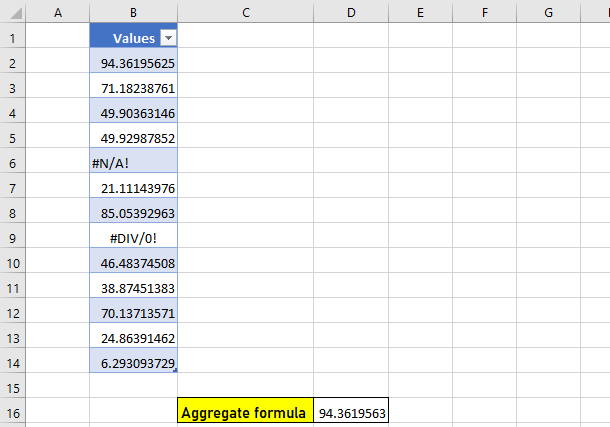
So as you can see some data has been given in column B which we will find the maximum value of the cell with the help of aggregate formula
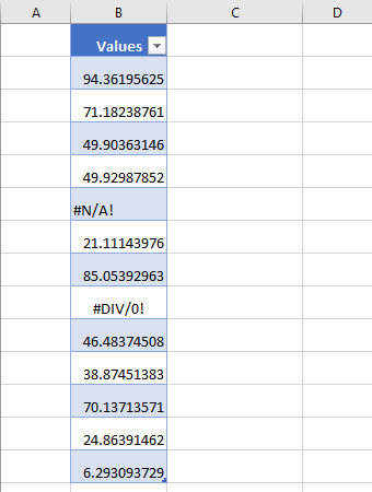
But if we use MAX formula to find the maximum value then error value is given in the cell due to which we will get value error only then we will use aggregate formula,
=AGGREGATE(4,6,Table2[Values])
In the formula, 4 is being used for max value and 6 for ignore error value.
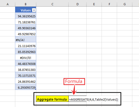
After using the formula, we will enter and find the result by ignoring the error value.
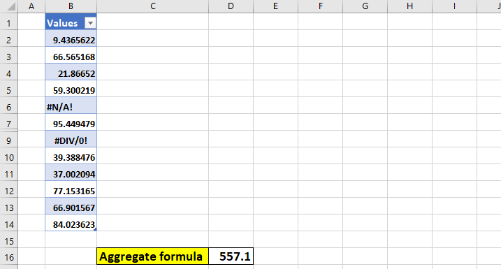
Make Total and ignore errors
So as you can see there is some data given in column B which we will be able to calculate the sum of the cell with the help of total formula.
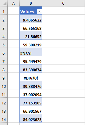
But if we use sum formula to find total value then error value is given in cell due to which we will get value error only then we will use aggregate formula,
=AGGREGATE(9,7,Table1[Values])
In the formula, 9 is being used for sum value and 7 for ignore hidden value and error value.
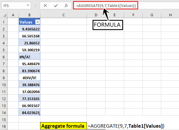
After using the formula, we will enter and find the result by ignoring the hidden value and error value.
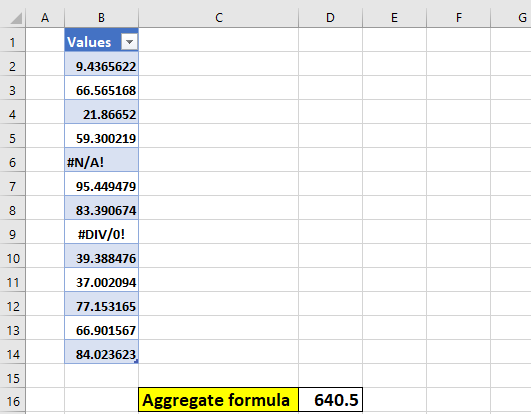
We will do one more operation for ignore hidden value and error value which will show hidden so now if we hide row 8 then our result will change
There is no new formula for hidden row because here already hidden value and error value formula has been used, so we can see that the value of total is changing by removing the row.
DOWNLOAD USED EXCEL FILE FROM HERE>>
So I hope you have understood this formula and for more information, you can follow us on Twitter, Instagram, LinkedIn, and YouTube as well.
You can also see well-explained video here
