Welcome to Excel Avon
Vertical Bullet chart in Excel
DOWNLOAD USED EXCEL FILE FROM HERE>>
In today’s post we will show you how to Create Vertical Bullet chart in excel, although it is quite simple, Excel Vertical Bullet Chart is one of the best ways to represent performance-related data in Excel. Use it to display the performance achieved in various parameters and compare it against the set target. You can make it vertical or horizontal depending on the work.
This comes in very handy when you need to display performance charts in a space-constrained Excel dashboard. In this article, I will teach you how to create Vertical Bullet Chart in Excel step by step with pictures.
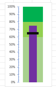
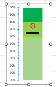
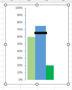
By the way, our Vertical Bullet chart is going to be like this as you can see.
Create Vertical Bullet chart in Excel
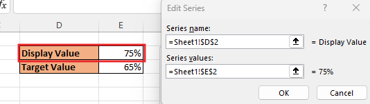
Create a table in excel sheet which will look something like this. where the data is something like this. First of All, we have to set some levels which sum will be 100.
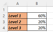
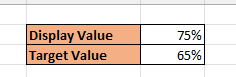
Here an average score of 65% is targeted, but you are given 75% as the display score.
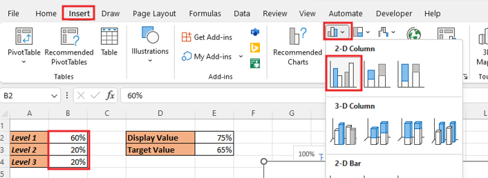
Select the data, then go to ‘Insert‘ Tab. Insert the chart by going to the ‘Insert‘ Tab.
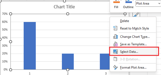
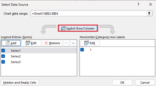
Right click on the chart will Data Selection. Here we will click on the Switch Row/Column Bottom.
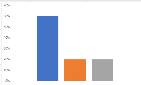
Now we will remove the Elements from the chart.
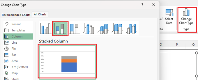
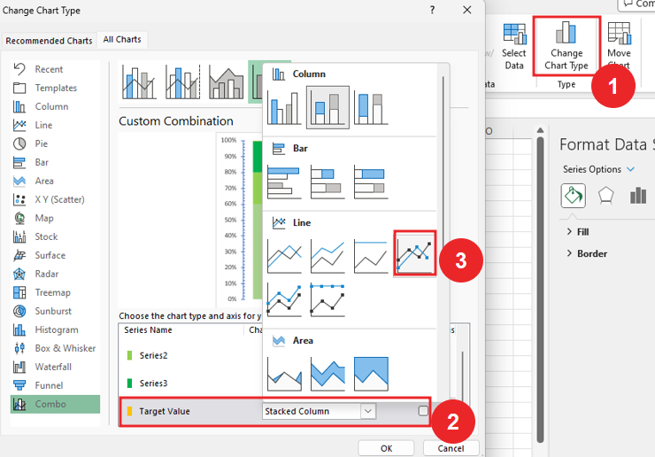
Right click on the Column and go to the Change Chart Type.
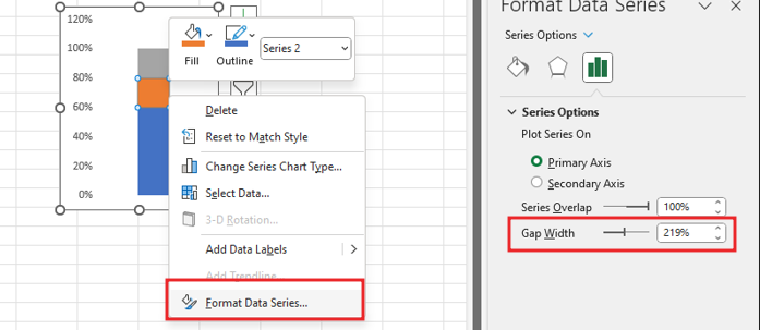
Now we will right click on the chart then go to ‘Format data Series‘. If you reduce the gap width of the chart, then the width of the chart will increase.
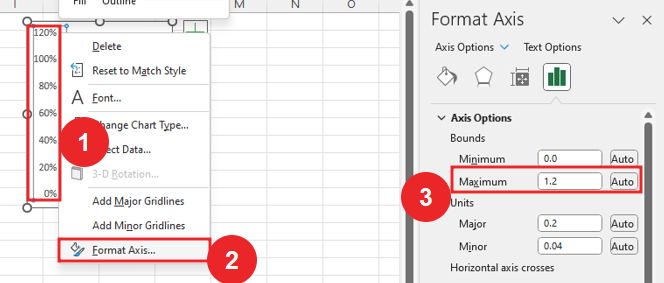
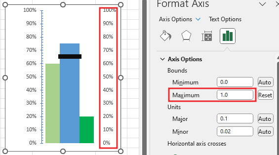
Right click on the axis of the chart and then click on Format Axis Option. Change the max value of Bound from 1.2 to 1.
We will add tick marks to the axis, let the major type be outside and the minor type be inside.
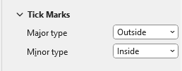
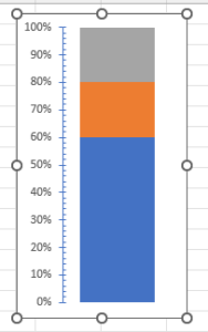
Now you can see in axis here inside and outside tick has been added as well as scale value has changed from 120 to 100.
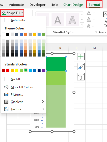
Now we will do the color formatting of the chart, first right click in the chart column, then go to the format option, here go to the shape fill option and fill the color according to your own, for all the levels, you will do the same color.
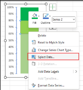
Right click on the chart go to select data option.
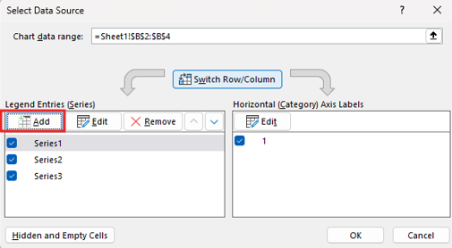
Click the add Button here we have to add series name and series value.
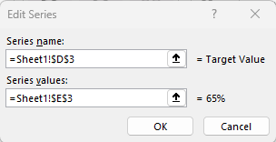
Put the Series name ‘Target Value’ , The Value of target value cell is added to the series value.
‘ 
Target value graph is added but not shown. SO then click on chart then go to ‘Change Chart type’ then change the type of chart to ‘Line with Marker’ for the Target Value graph.
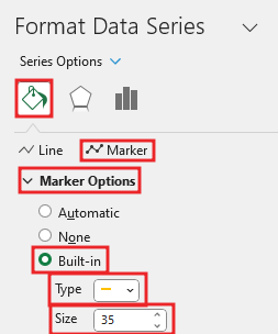
There is a mark in the chart which is of ‘target value’. Formatting will be done by right clicking this point with format data series option. First go to the fill option then select the markers, go to the markers option, go to the built in option and change the type and increase the size of markers from here.
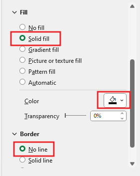
Fill the marker solid and then change the color. ‘No line’ the markers Border.
Right click in the chart the go to ‘Select data’ option.
Click the add Button here we have to add series name and series value.
Put the Series name ‘display Value’, The Value of Display value cell is added to the series value.
The display value marker has been added to the chart.
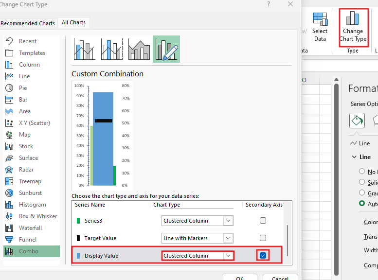
First of all go to the fill option then select the markers, go to the markers option, go to the built in option, from here we will change the type and size, here we will also add the secondary axis.
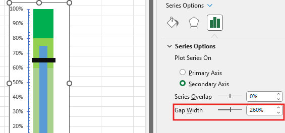
Click on the chart will go to format data series option, Increase the gap width.
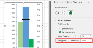
Now we will right click on the secondary axis then go to ‘Format data Series‘. If you increase the gap width of the chart, then the width of the chart will reduce 0.8 to 1.
Now delete secondary axis.
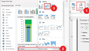
Click on the graph with Series 1, go to Change Chart Type. Here we will open the dropdown of Series 1 and select Stacked Column from here.
Now we will right click on the chart then go to ‘Format data Series‘. increase the width Gap.
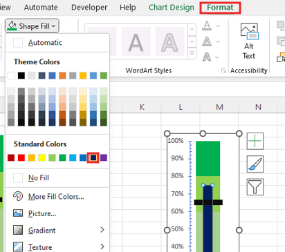
Now we will change the color by going to shape fill.
Now our Vertical Bullet chart is ready.
Therefore, I hope that you have understood How to create Vertical Bullet Chart in Excel, maybe if you do not understand anything, then you can comment us with the question, which we will answer soon and for more information, you can follow us on Twitter, Instagram, LinkedIn and you can also follow on YouTube.
DOWNLOAD USED EXCEL FILE FROM HERE>>
LEARN MORE DASHBORAD AND CHART TOPIC HERE
You can also see well-explained video here about How to create Vertical Bullet chart in Excel


