Welcome to Excel Avon
Timer Chart in Excel
DOWNLOAD THE USED EXCEL FILE FROM HERE>>
In today’s post we will tell you how to make timer chart in excel, yes it may be little different here we will use shape for timer chart also use 2-D pie chart with shapes it is very simple, excel timer chart The circle looks like a progress chart. Timer Chart Will Give You a Very Professional Feel This chart, although not commonly used, but it looks like a stop watch, is a great way to present time-related data. Technically, several shapes would be used to create a timer chart, and then a 2-D chart would be used.
In this article, I will teach you to create timer Chart in Excel step by step with pictures.
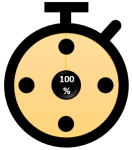
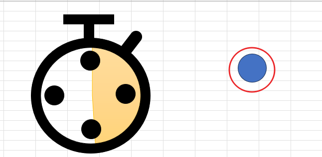
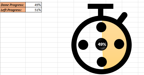
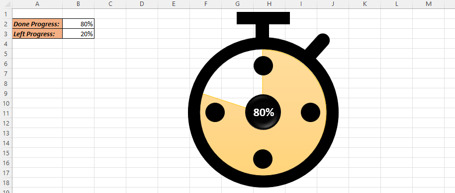
Well, as you can see, our timer chart is going to be like this.
Create Timer Chart in Excel
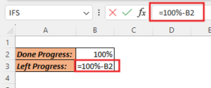
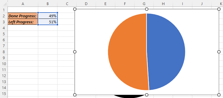
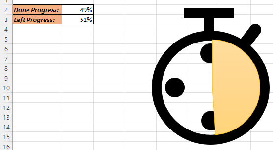
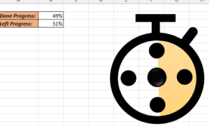
Create a table in excel sheet which will look something like this. In which there will be 2 Values. Done progress and Left Progress. Added formula for Left Progress =100%-B2.
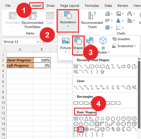
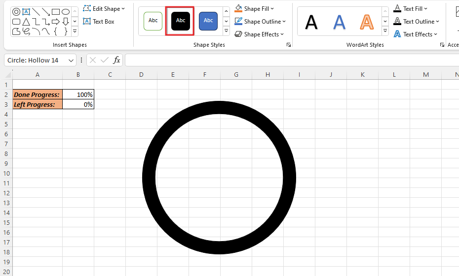
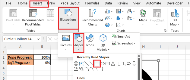
Without selecting any data, insert a circle Hollow shape by going to insert tab> Illustrations> Shapes> Basic Shape > Select Circle Hollow.
Drag the select shape in the sheet, yes many of you will think this is a doughnut chart which is not really it is a shape which looks like a doughnut chart.
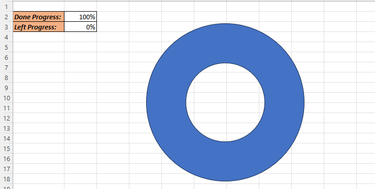
After drawing this chart, you increase the hole size of the shape by dragging the yellow point visible in the shape.
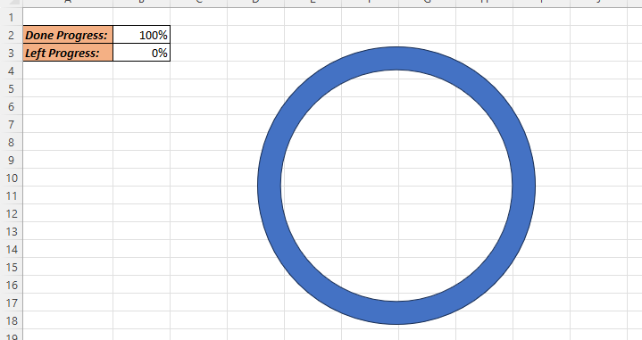
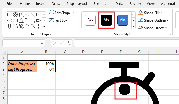
The color of the shape will change with the shape style.
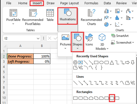
Now Insert rectangle shape by going to insert tab> Illustrations> Shapes
Drag the select shape in the sheet and fit the rectangle shape as like you see that in picture. Exactly as if in the middle of the circle, change the color of the shape. And copy and paste shape because 2 shapes have been added Yes, the chart handles may be slightly misaligned.
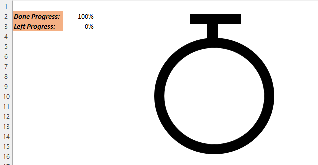
Without selecting any data, insert another rectangle shape having rounded top corners. Insert shpae by going to insert tab> Illustrations> Shapes> Rectangle shape.
Drag the select shape in the sheet and make the top corner of the shape full round as like you see that in picture.
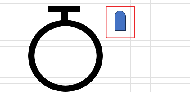
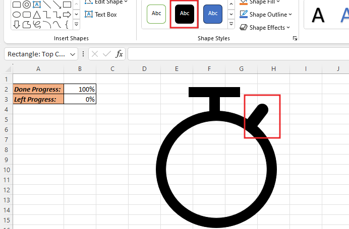
And now add the shape with circle or dial of timer chart, you can shrink the shape a bit so that it will fit in the circle. The color of the shape will change with the shape style with No Outline.
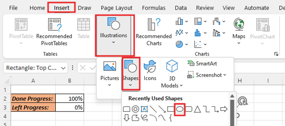
Now we will Insert Oval shape by going to insert tab> Illustrations> Shapes> Oval shape.
Drag the select shape in the sheet with shift key for perfect rounded circle as like you see that in picture.
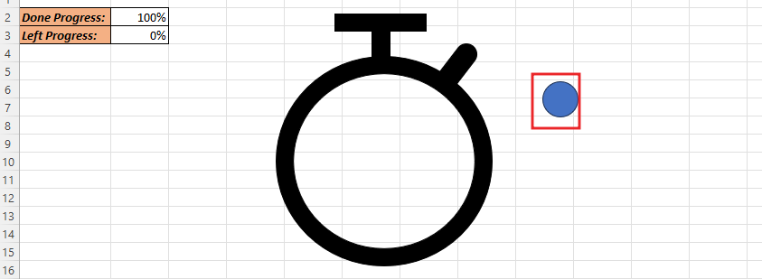
Now you have to shift the created circle shape inside the dial of the timer, after that you change the color of the shape with the shape style.
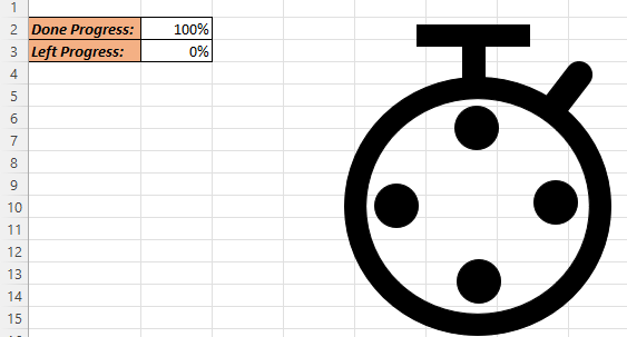
Make three copies and shift them inside this dial as shown in the image.
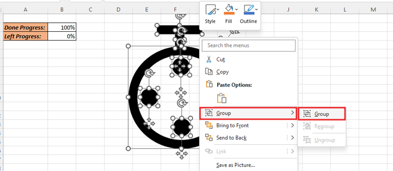
Then Select all the shape and right click then group them.
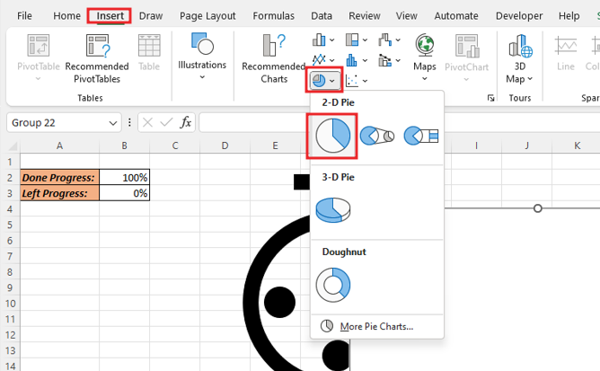
Now we will insert 2-D Pie Chart by going to Insert tab.
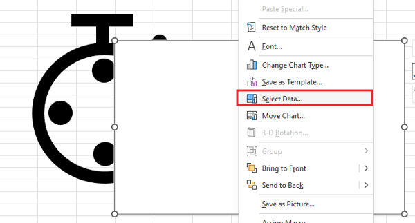
Right click on the chart then go to Select data Option.
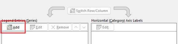
Click the add Button Give the name of series give the value of series. For series value you select Cell Cone progress and left progress.

Now Delete the legend and chart title from the chart.
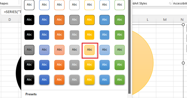
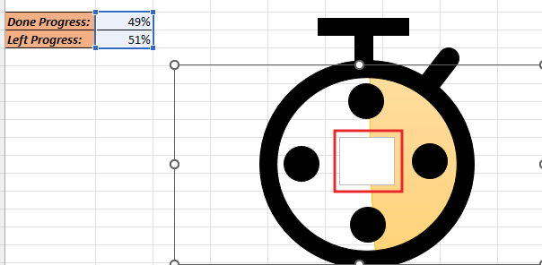
Now fill the orange part by shape Fill, Make the Background of the 2-D pie chart NO Fill with shape fill and No Outline.
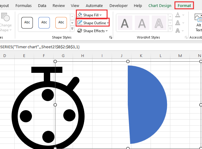
And now change the theme style of blue part.
Make 2-D pie chart equal to Circle size, 2-D pie chart overlays in circle.
 \
\
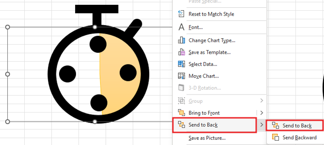
Right click on the chart then go to send to back Option so that the 2-D pie chart will be circled.
Now we will Insert Oval shape by going to insert tab> Illustrations> Shapes> Oval shape.
Drag the select shape in the sheet with shift key for perfect rounded circle as like you see that in picture.
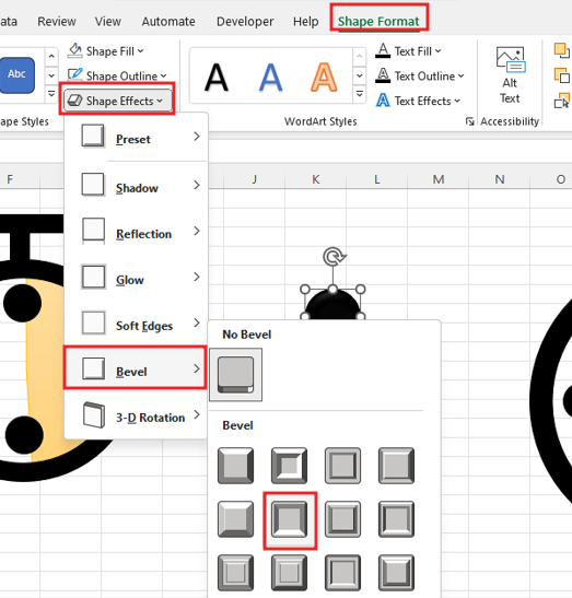
Created circle black with shape style and then add effect to the shape.
Now pick the shape and shift it to the circle.
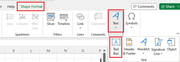
Go to insert tab and select it in the text box and drag it over the shape align text box.
Now remove the background and outline of the text box by going to the Format option with No Fill and No Outline.
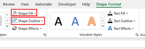
Add formula in Text Box =B2. after aligning the text box. Customize text box, Bold, size of font color, size of font.
Then Select all the shape and right click then group them.
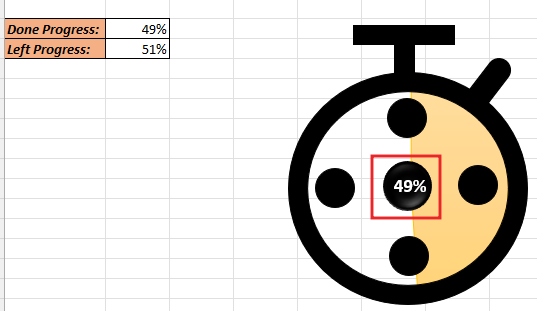
Now you can check the chart and change the value.
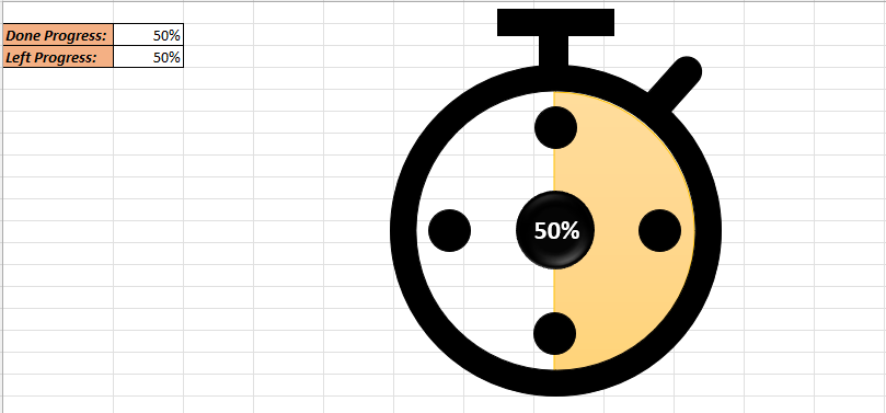
Now our Create Timer Chart in Excel.
Therefore, I hope that you have understood How to Create Timer Chart in Excel, maybe if you do not understand anything, then you can comment us with the question, which we will answer soon and for more information, you can follow us on Twitter, Instagram, LinkedIn and you can also follow on YouTube.
DOWNLOAD THE USED EXCEL FILE FROM HERE>>
LEARN MORE DASHBORAD AND CHART TOPIC HERE
You can also see well-explained video here about How to Create Timer Chart in Excel


