Welcome to Excel Avon
Funnel Chart in Excel
DOWLOAD THE USED EXCEL FROM HERE>>
In today’s post we will show you how to Create Funnel chart in excel, although it is quite simple, Funnel charts are great for visualizing a store of data moving from one stage to the next. With your data in hand, we’ll show you how to easily add and create a funnel chart in Microsoft Excel. As the name implies, a funnel chart has its largest section at the top.
Each subsequent section is smaller than its predecessor. Seeing the largest gaps allows you to quickly identify stages in a process that can improve.
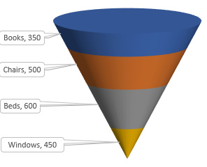
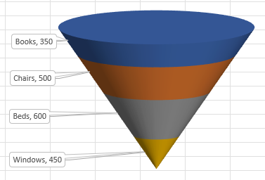
By the way, our Funnel Chart is going to be like this as you can see.
Create Funnel Chart in Excel
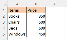
Create a table in excel sheet which will look something like this. where the data is something like this.
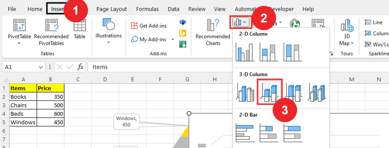
Go to insert tab then click on Insert tab and insert the chart.
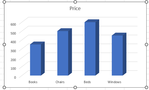
we have inserted the chart, but our chart is something like this.
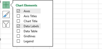
Remove the ‘Data Labels’ and Keep ‘Axes’
Now we’ll change the type of chart.

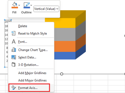
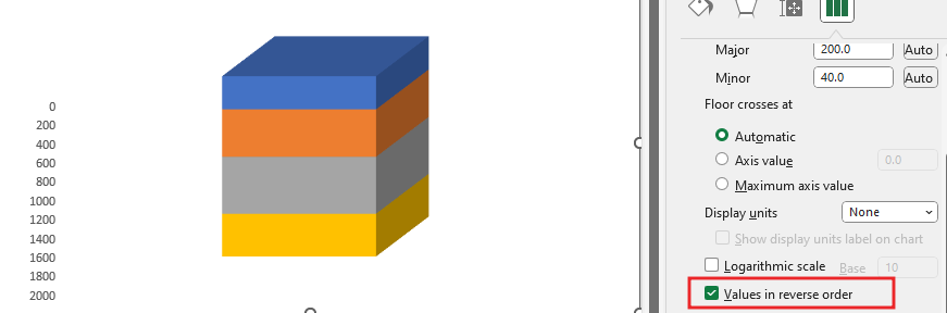
Right click on vertical axes. Click format axis, then reverse order the value.
Then reverse order the value after this our chart will be in reverse order as you can see after this, we will remove axes.
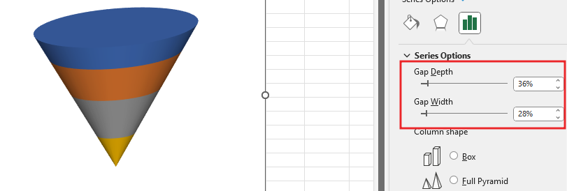
Now we will go to format data series option by right click and then we will select full Cone shape.
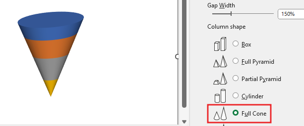
In full Cone shape we will reduce gap depth and gap width.
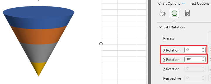
Right click on chart and Go to ‘3-D Rotation‘ Option then change X Rotation and Y Rotation
Add data label one by one to all parts of chart (For this, right click on the chart and click on ‘Add Data label’ option)

Select Each Data label and right click on it, go to ‘Format Data Label‘ and click on ‘Series Name‘ option.
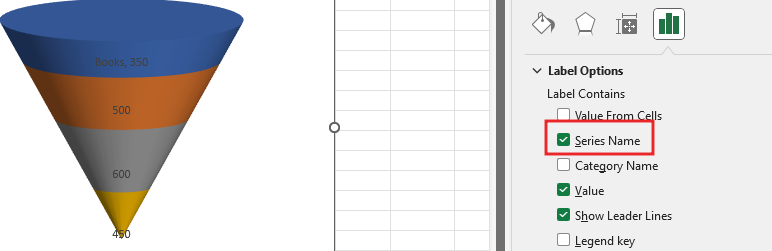
Similarly add series name for all the labels.
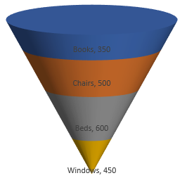
We Changed the shape of all the data labels one by one. Do some changes according to the chart to make it look good. (Follow the video)
Therefore, I hope that you have understood How to create Funnel Chart in Excel, maybe if you do not understand anything, then you can comment us with the question, which we will answer soon and for more information, you can follow us on Twitter, Instagram, LinkedIn and you can also follow on YouTube.
DOWLOAD THE USED EXCEL FROM HERE>>
LEARN MORE DASHBORAD AND CHART TOPIC HERE
You can also see well-explained video here about How to Create How to create Funnel chart in Excel


