Welcome to Excel Avon
Circle Bullet chart in Excel
DOWNLOAD THE USED EXCEL FILE FROM HERE>>
In today’s post we will show you how to Create circle Bullet chart in excel, although it is quite simple, Excel circle Bullet Chart is one of the best ways to represent performance-related data in Excel. Use it to display the performance achieved in various parameters and compare it against the set target. You can make it vertical or horizontal or circle depending on the work.
This comes in very handy when you need to display performance charts in a space-constrained Excel dashboard. In this article, I will teach you how to create circle Bullet Chart in Excel step by step with pictures.
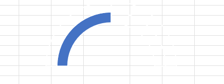
By the way, our circle Bullet chart is going to be like this as you can see.

Create Circle Bullet chart in Excel
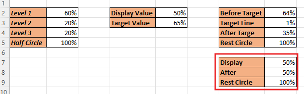
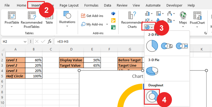
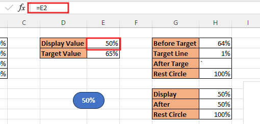
Create a table in excel sheet which will look something like this. Our main chart will be made from this table data. This Whole circle will be in 4 parts, which will display all separately.
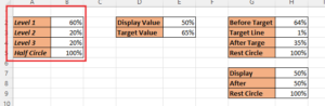
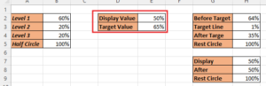
The second is the data display the the target value that will display the value.
Third data we’ve added for the target line. In ‘Before target‘ value we subtract 1 from the target line.
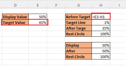
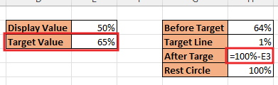
Subtract the ‘Target Value’ from 100 to the value of the ‘After Target’ cell.
In fourth data, add the display value for display and subtract the ‘Display’ cell from 100 to the value of the ‘After’ cell.
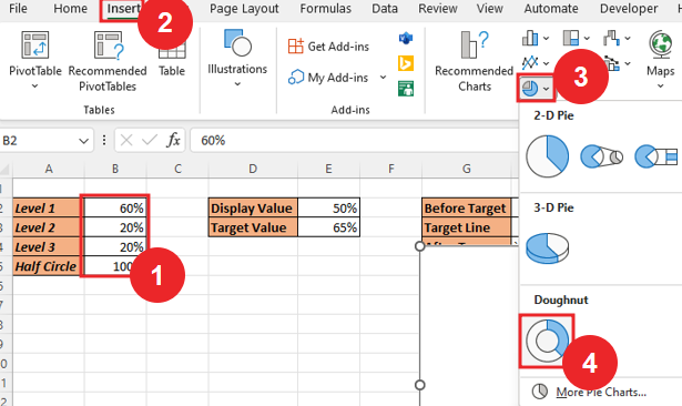
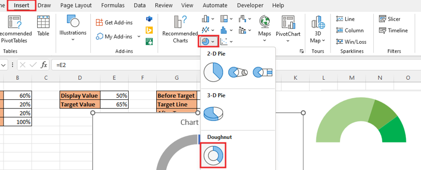
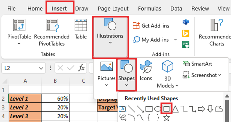
Select the First data table, then go to ‘Insert‘Tab. Insert the Doughnut chart.
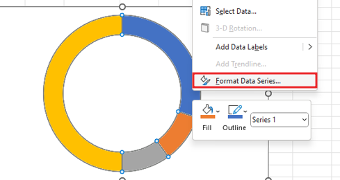
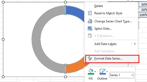
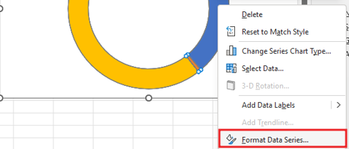
Delete legend and title from chart. Right click on the chart GO to Format data series option.
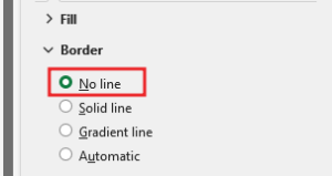
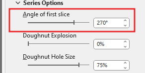
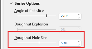
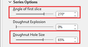
Make the border ‘No line’ and rotate 270* Angle of first slice. Reduce hole size of the chart.
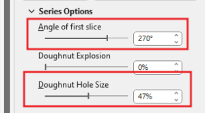
Now the lower part of chart 50% No Fill it with format option this 50%-part is rest part.
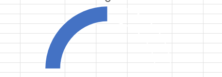
Now from format option, fill all parts with different color. After color formatting our chart will look like this. Now let’s turn this chart to the side.

Select the 4th data table, then go to ‘Insert‘Tab. Insert the Another Doughnut chart. You may not see the picture to select the data table, you will have to select the data and insert the chart.
Delete legend and title from chart. Right click on the chart Go to Format data series option.
Make the border ‘No line’ and rotate 270* Angle of first slice. Reduce hole size of the chart.
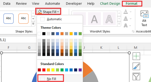
Now we’ll hide rest part and after part by ‘No fill‘ By going to Format >Shape Fill >No Fill.

After this we will select the chart and make it ‘No Fill‘ from the ‘Shape Fill‘ option and ‘No Outline’ from ‘Shape Outline‘.
Now we’ll copy second doughnut chart and paste it 2 times. After pasting you can see inner, middle and Outer doughnut chart.
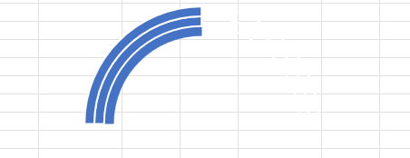
Going to the format option, we will make the inner and outer part ‘No fill‘.
Reduce the hole size of the middle doughnut chart. Right click on Chart then click on ‘Format data series’ then reduce size.
Now we can see that our chart is ready like this, now to insert new chart, second doughnut will move the chart side.
Select the 3rd data table, then go to ‘Insert‘Tab. Insert the Another Doughnut chart. You may not see the picture to select the data table, you will have to select the data and insert the chart. Once you select the 3rd data then you follow the steps given in the picture.
Delete legend and title from chart. Right click on the chart go to Format data series option. ‘No Line‘ the border of the chart.
Rotate 270* Angle of first slice. Reduce hole size of the chart.
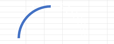
No-Fill all parts except the target line parts. You can see the chart before and after No fill and No Out Line.


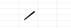
Color of the target line part black with shape Fill. No Fill in chart background by going to format >Shape Fill >No Fill.
Now select all charts and go to Shape format, align right by going to align Option, then align the middle.
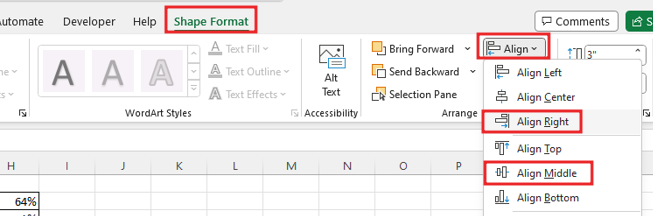
When all the charts are aligned then the Circle Bullet chart will look something like this.

From the insert option we’ll insert a shape.
Drag shape into the sheet. And add the formula to the shape =E2. Now whatever value is of E2 it will be printed in the shape.
You can customize the shape, align it, make it bold and change the font, and then fit it below your Circle bullet chart.

Therefore, I hope that you have understood How to Create Circle Bullet Chart in Excel, maybe if you do not understand anything, then you can comment us with the question, which we will answer soon and for more information, you can follow us on Twitter, Instagram, LinkedIn and you can also follow on YouTube.
LEARN MORE DASHBORAD AND CHART TOPIC HERE
You can also see well-explained video here about How to Create Circle Bullet chart in Excel


