Welcome to Excel Avon
Balance Chart in Excel
DOWNLOAD THE USED EXCEL FILE FROM HERE>>
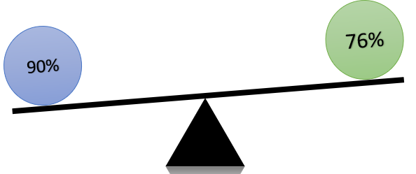
In today’s post we will show you how to make balance chart in excel, yes it may be a bit different here we will use shape for balance chart it is very simple, excel balance chart looks like a scale. This chart is a great way to represent performance-related data. Technically, the balance chart will be drawn with an oval shape and a straight line.
In this article, I will teach you to create Balance Chart in Excel step by step with pictures.
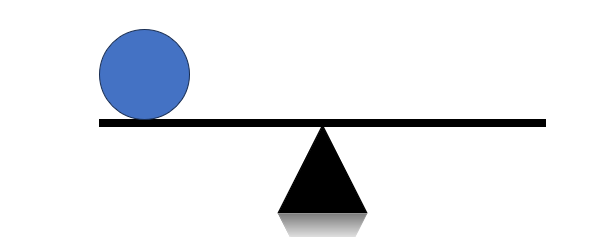
Well, as you can see, our balance chart is going to be like this.
Create Balance Chart in Excel
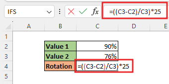
Create a table in excel sheet which will look something like this. In which there will be 3 parts Value 1, Value2 and Rotation. Added formula for rest part. ==((C3-C2)/C3) *25, Rotation cell convert it to general format.
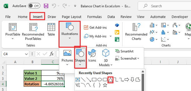
Go to Insert tab> Illustrations> shapes> Pick Triangle. and then drag triangle with shift in worksheet.
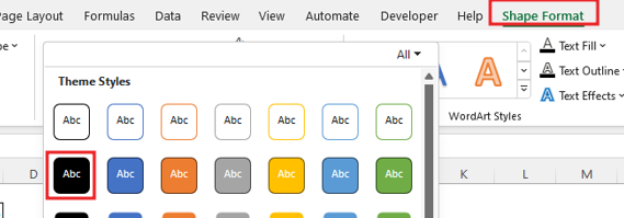
Fill Black color in triangle with themes style. add reflection effect to triangle.
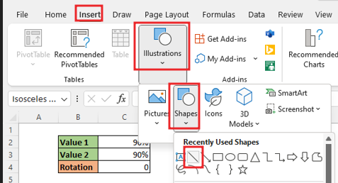
Again, go to Insert tab> Illustrations> shapes> Pick straight line. and then drag line with shift in worksheet.
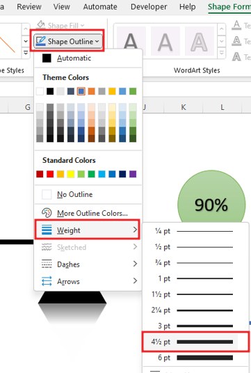
Increase the line weight by going to the shape outline. Select color for line with themes style.
We will center align by selecting the created triangle and line.

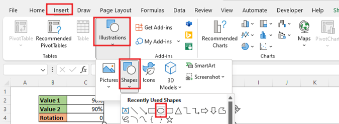
Again, go to Insert tab> Illustrations> shapes> Pick Oval shapes. and then drag Oval with shift in worksheet.
When you have dragged the oval, then we will keep the oval shape adjacent to the dragged line, like this image is given below.
Now we will color fill the created circle or oval shape, you can fill any color as we are doing by going to the shape format.

Then we will add formula in oval shape. After adding the formula, whatever value is in cell C2 will be filled in shape 1. Format the text in the shape, make the text bold, increase the size or change the color.

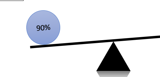
With shape format, you can add any style to the text from wordArt style.

Copy and paste shape 1 to other end of line. Keep ovel 2 adjacent to the line. change the formula in oval2. =C3 After adding the formula, whatever value is in cell C3 will be filled in shape 1. The chart will now look something like this.
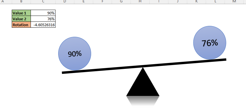
Format the text in the shape and change the color of oval 2 by going to Shape format.
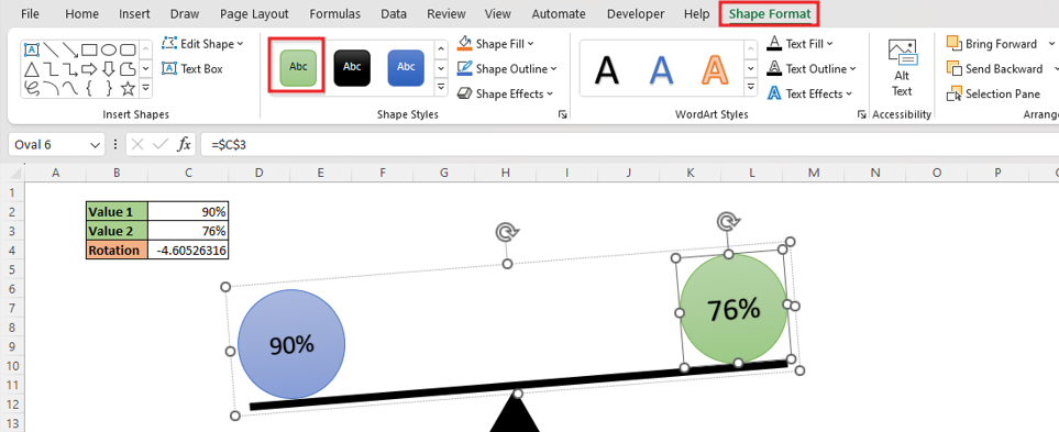
Now make the group by selecting the line, oval 1 and oval 2.
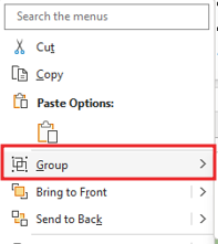
Now copy the group name and click Alt+F11 for open VBA sheet.
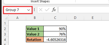
When you see in the sheet, then there will be a sheet in general mode at the top, you can convert it from general to worksheet.

We will change the procedure from selection change to just change. then we ‘change’ this subroutine will automatically be defined in the sheet.
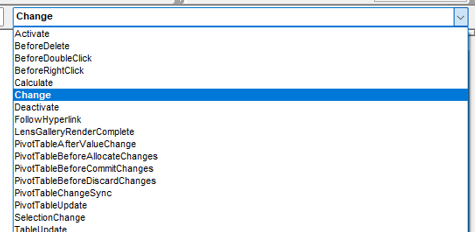
Delete the selection change subroutine from the sheet. and write code for rotation of group 7. Add the range of the rotation cell to the code.
Private Sub Worksheet_Change(ByVal Target As Range)
Me.Shapes("Group 7").Rotation =  Me.Range("C4").Value
End Sub
Change the value of cell. then the chart will be change.
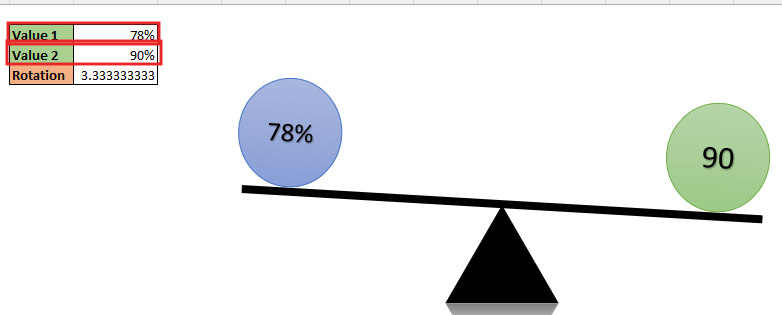
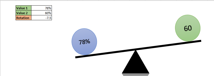
This balance chart has minimum value is 25%. If you have any difficulty to understand this balance chart so you can comments us.
Therefore, I hope that you have understood How to Create balance chart in Excel, maybe if you do not understand anything, then you can comment us with the question, which we will answer soon and for more information, you can follow us on Twitter, Instagram, LinkedIn and you can also follow on YouTube.
DOWNLOAD THE USED EXCEL FILE FROM HERE>>
LEARN MORE DASHBORAD AND CHART TOPIC HERE
You can also see well-explained video here about How to Create Balance chart in Excel


