Welcome to Excel Avon
3-D Pie Chart in Excel
DOWNLOAD THE USED EXCEL FILE FROM HERE>>
In today’s post we will show you how to Create 3-D Pie chart in excel, although it is quite simple, Excel has a long range of options to make different types of charts. The pie chart is one of the most common types of charts.
A pie chart shows the data in proportion to a whole. The 3D pie chart consists of a circle that is divided into segments, each representing a proportion of the share of each value in a dataset.
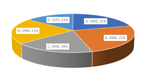
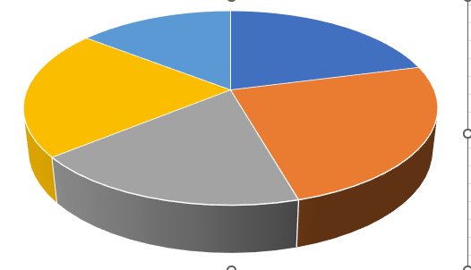
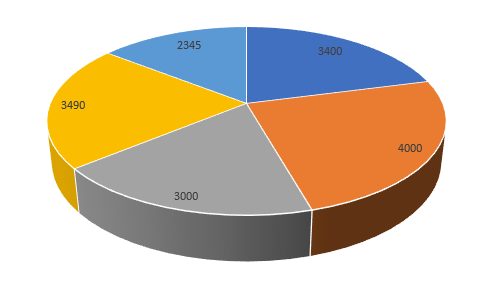
By the way, our 3-D pie Chart is going to be like this as you can see.
Create 3-D Pie Chart in Excel
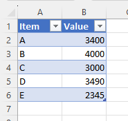
Create a table in excel sheet which will look something like this. where the data is something like this.
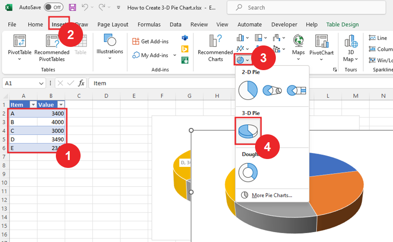
First, select the entire dataset then Go to Insert Ribbon and insert the chart.
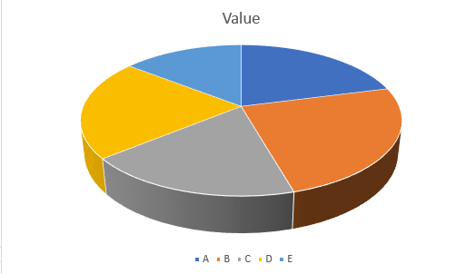
we have inserted the chart, but our chart is something like this.
After that, click on the Chart Title and remove it as with labels.
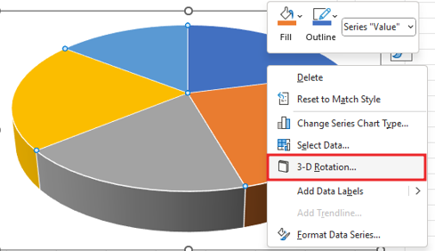
Right click on chart. then click on 3-D Rotation.
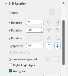
Here we will customize the x rotation, y rotation and perspective of chart. perspective can also be increased by up and down buttons.
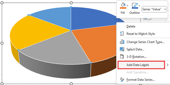
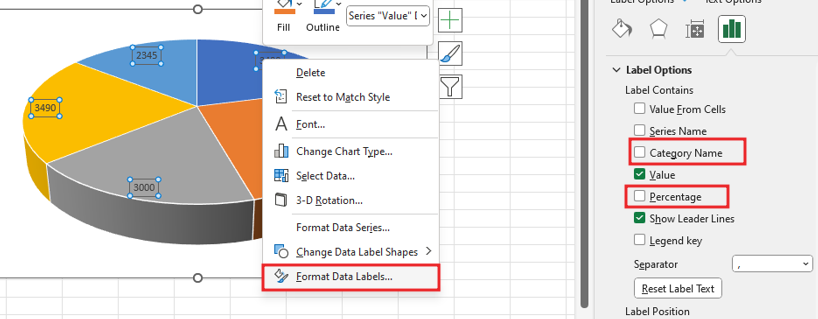
Again, right click on chart and add data labels.
After the data labels are added
Right click on Data Labels then go to Format Data Labels and add elements to the labels like Percentage and Category Name.
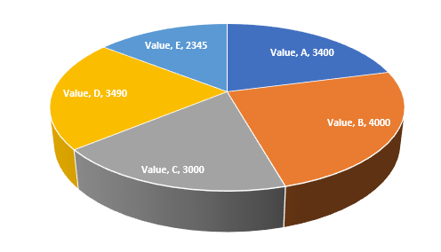
Tick the percentage and category name so that they will be added, after selecting the chart will become like this.
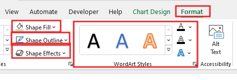
To select the labels, you will go to the Format tab, from here you can format the labels, fill the shape, add outline or effect to the shape, and also change the font style.
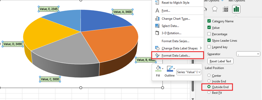
If we want to remove these labels from the top of the chart and bring them to the side, then we will right click on the labels, go to Format Data Labels, then scroll down, we will go to the option Labels position and select it outside end.
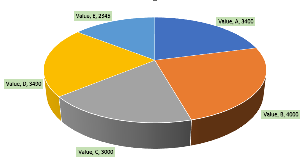
Labels is off the charts now and our chart is ready.
Therefore, I hope that you have understood How to create 3-D Pie Chart in Excel, maybe if you do not understand anything, then you can comment us with the question, which we will answer soon and for more information, you can follow us on Twitter, Instagram, LinkedIn and you can also follow on YouTube.
DOWNLOAD THE USED EXCEL FILE FROM HERE>>
LEARN MORE DASHBORAD AND CHART TOPIC HERE
You can also see well-explained video here about How to Create How to create 3-D Pie chart in Excel


