Welcome To Excel Avon
With conditional formatting Highlight Top or Bottom value in Excel
The best way is to highlight top or bottom values with the help of conditional formatting. Top values are Maximum values in list and bottom values are minimum values in list. It is very fast and simple and you will just follow few steps, in this way we can highlight top values and bottom values without using any formula. We are Explain 2 example of Highlight Top or Bottom.
DOWNLOAD USED EXCEL FILE FROM HERE>>
Highlight top 10 values with Conditional Formatting
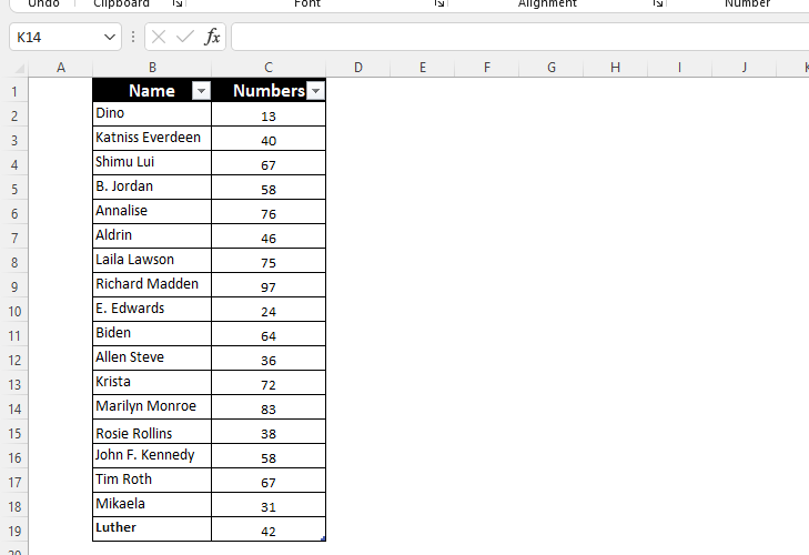
As you can see we have data showing some ways to highlight from top to bottom. In which the marks obtained by some students in the subject, we will highlight the top 10 students and show which students got the top 10 marks.
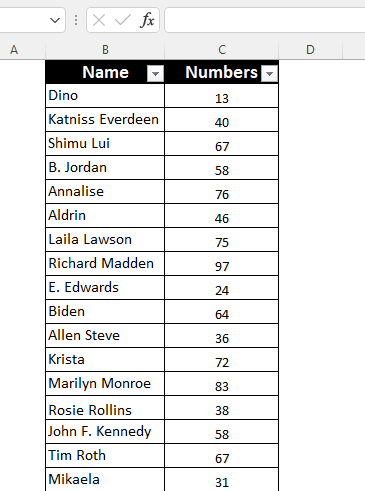
Select the cell or range C2:C19 highlight for number
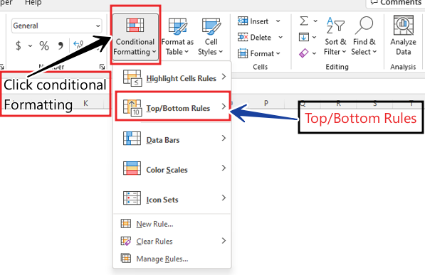
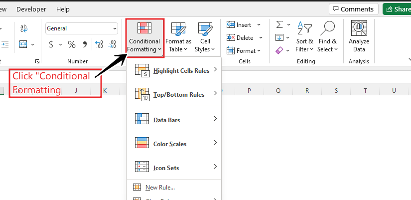
Click the conditional formatting icon in from home menu ribbon, Now we will select the top/bottom rules from the drop down menu, Select the top 10 Items from the menu.
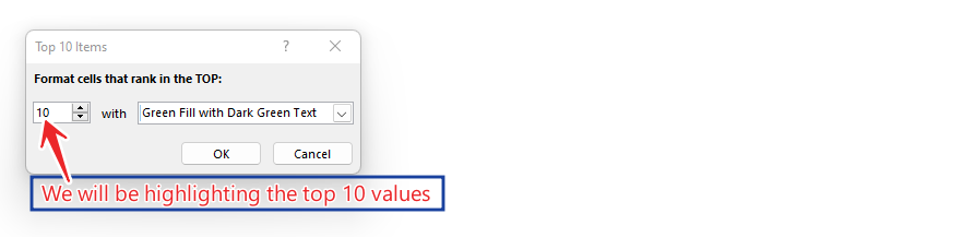
After clicking in Top 10 a dialog box will open where you can specify the value and appearance options.
Leave the default value 10 in the input field as we will be highlighting the top 10 values
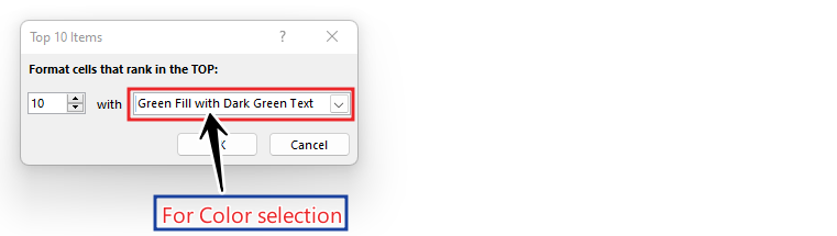
Select the Appearance option “Fill green with dark green text” from the dropdown menu
Now you can see that the 10 cells with the top 10 values will be highlighted in green

Now, you can easily identify the marks obtained by top 10 students.
Note: The default number of items is 10, but you can specify any whole number up to 1000 for Top or Bottom Items to be highlighted.
Highlight Bottom 10 values with Conditional Formatting
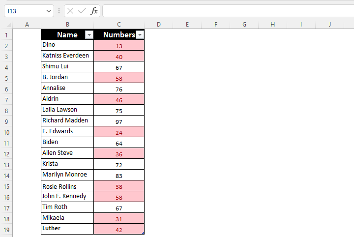
As you can see we have data showing some ways of highlighting from top to bottom. In which the marks obtained by some students in the subject, we will highlight the bottom 10 students and show which students have scored the bottom 10 marks.
The “bottom 10” rule, step by step:
Select the range C2:C19 for the subject score.
Home Tab>Conditional Formatting Icon
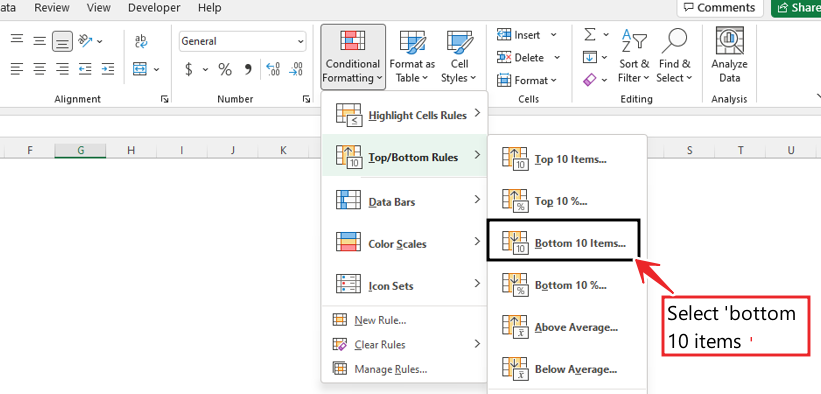
Select Top/Bottom Rule from the drop-down menu, Select Bottom 10 Items… at the bottom of the menu.
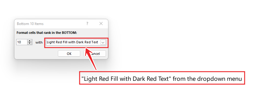
This will open a dialog box where you can specify the value and appearance options.
Leave the default value 10 in the input field
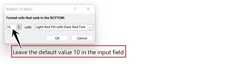
Select the appearance option “Light Red Fill with Dark Red Text” from the dropdown menu
Now, you can see that the bottom 10 students will be highlighted in red:
So you must have understood the Highlight Top or Bottom in Excel
So I hope you have understood this Highlight Top or Bottom in Excel and for more information, you can follow us on Twitter, Instagram, LinkedIn, and YouTube as well.
DOWNLOAD USED EXCEL FILE FROM HERE>>
You can also learn about highlight duplicates in excel
You can also see well-explained video here
")

