Welcome to Excel Avon
Highlight Duplicates in Excel
DOWNLOAD USED EXCEL FILE FROM HERE>>
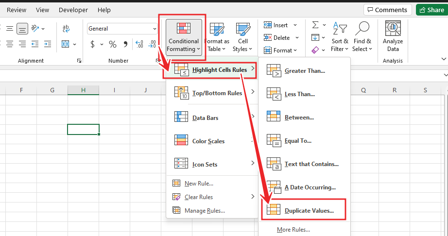
Using Duplicate Highlight, we can highlight any duplicate value, that data can be of any type as data can be given in row or column. To use Duplicate Highlight select the data from where we need to highlight the duplicates then we will go to Conditional Formatting which you can see on the Home tab then choose Duplicate Values option which is under Conditional Formatting.
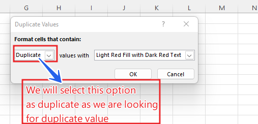
From the Duplicate Values box, select Duplicate with the type of color formatting we want. Red text is selected by default to highlight duplicates.
1) Highlight Duplicate Value Cells
The first example is for Highlight Duplicate Value Cells in which duplicate cells will be highlighted. So let’s see the example, then let’s see how it will highlight duplicates value.
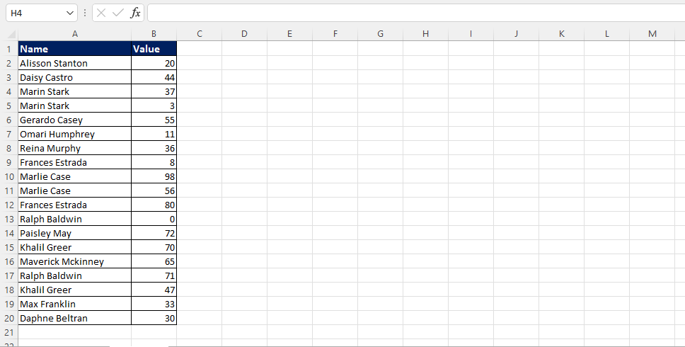
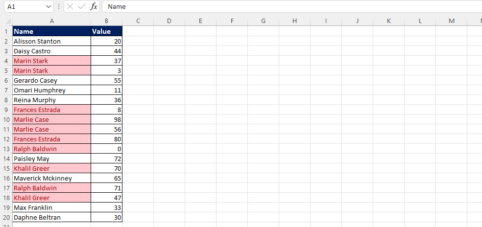
So as you can see above image, some of these cells have duplicate data, so we will highlight duplicates. First we will select that column or row
HOME TAB>CONDITIONAL FORMATTING>HIGHLIGHT CELL RULE>DUPLICATE VALUE
This will open a dialog box of duplicate values, see image below
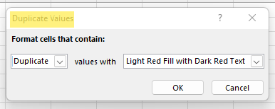
Select a color from the Color cell to highlight the cells
will highlight all the duplicate values in the given data here. Result is in below image.
I hope you have understood how to use these Highlight Duplicate Value Cells.
2) Highlight Duplicate Whole Row
Highlight Duplicates in Excel
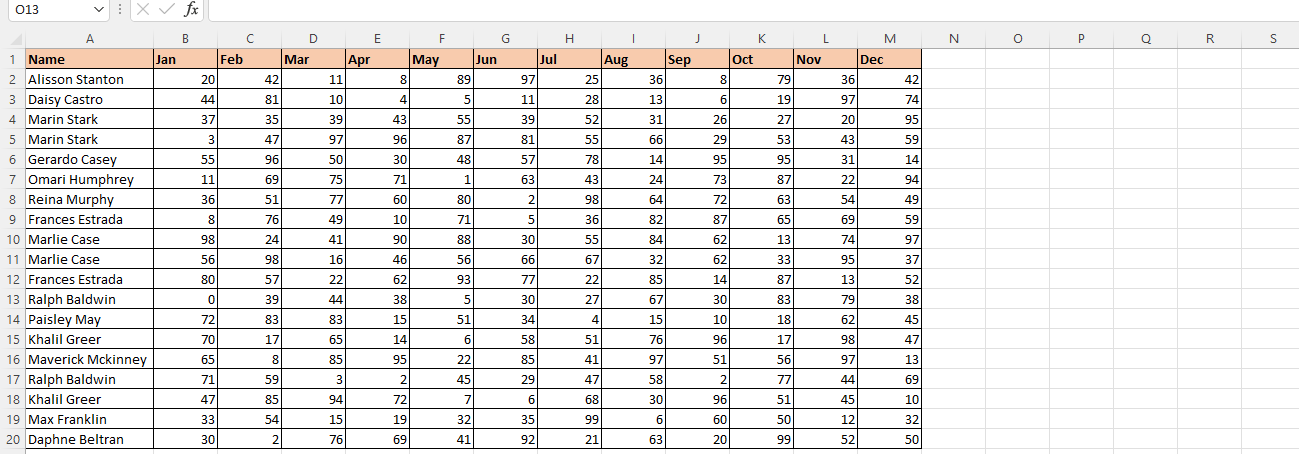
To find the duplicate ROW in Excel again let’s assume the new dataset. To highlight duplicate values here, we will use the COUNTIF function here which returns TRUE if the values appear more than once.
COUNTIF function,
=COUNTIF(starting cell range, cell address)>1
follow the steps
Select the entire data table.
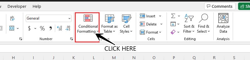
Go to the Home tab and click on the Conditional Formatting option.
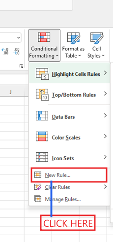
It will open a drop-down list of formatting options, Click on the New Rule option here.
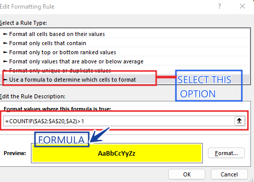
Open a dialog box for creating a new custom rule here, Select the last option, “Use a formula determining which cells to format”, under the Select a Rule Type section. And use this COUNTIF formula
=COUNTIF($A$2:$A$20,$A2)>1
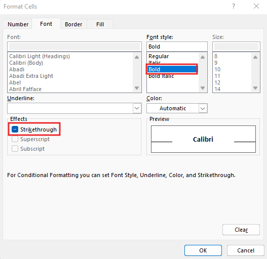
Go to format Choose the Fill color from the color palette for highlighting the cells, and then click on OK.
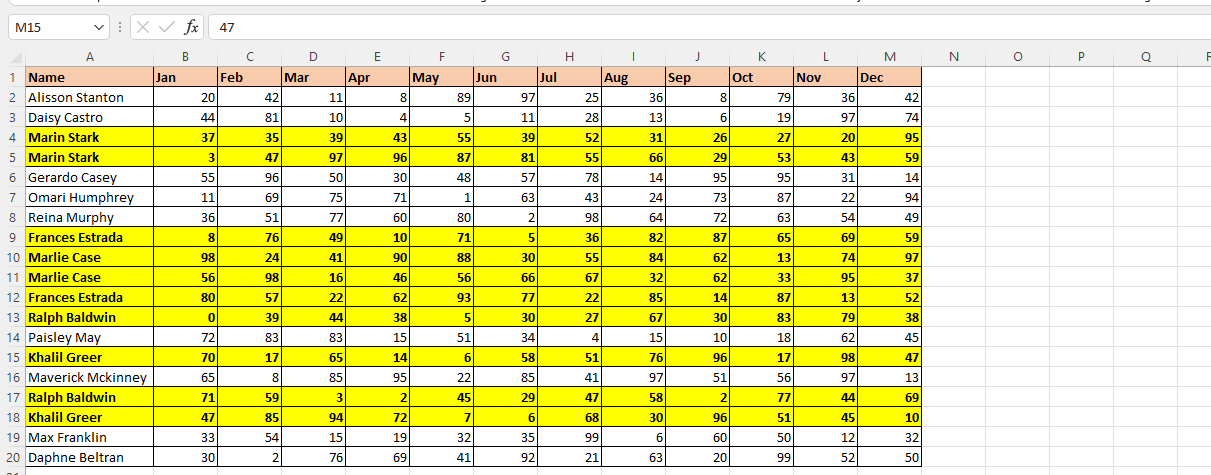
This will highlight all rows with duplicate values in the dataset. As you can see the image is given below
DOWNLOAD USED EXCEL FILE FROM HERE>>
So I hope you have understood this formula and for more information, you can follow us on Twitter, Instagram, LinkedIn, and YouTube as well.
You can also see well-explained video here
")
