Welcome to Excel Avon
What is a Color Scale
In Excel, we use the color scale when highlighting a range of cells, first for the minimum value and second for the maximum value. Between the minimum and maximum values, a gradient color scheme is used by mixing the colors for the minimum and maximum values. You can apply this to each individual row using conditional formatting. In this article, I will show you how to apply the Per Row Conditional Formatting Color Scale in Excel. Using this option only makes sense if you have a range of cells with lots of values and highlight an area.
How to use Color Scale
DOWNLOAD USED EXCEL FILE FROM HERE>>
2-Color scales
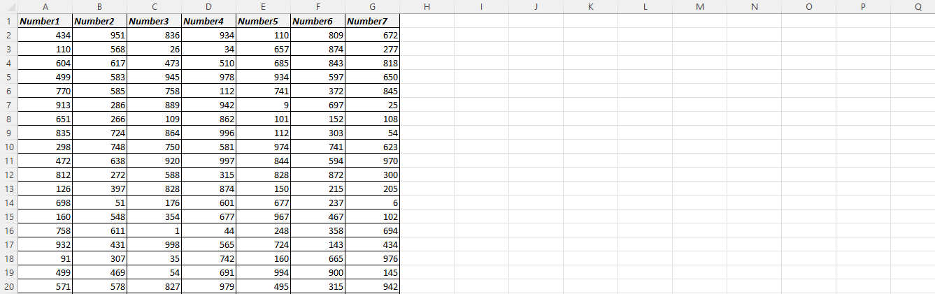
We have some data in which we will be using color scales. If you look in the excel sheet you will get the data, now we will do its color formatting.
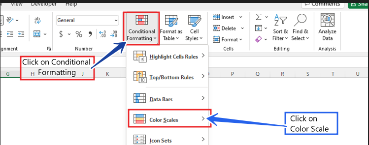
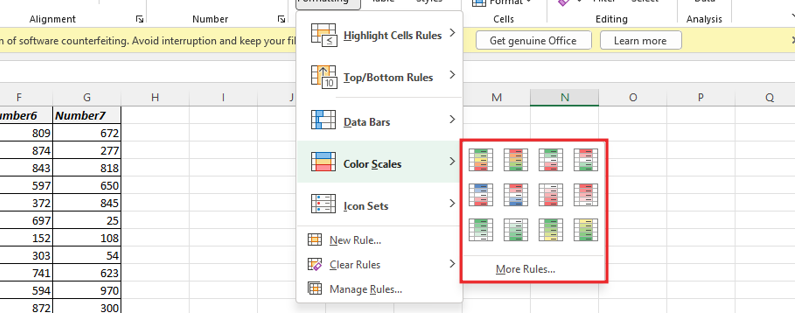
Select whole cell Activate, and click on Conditional Formatting > Color Scales
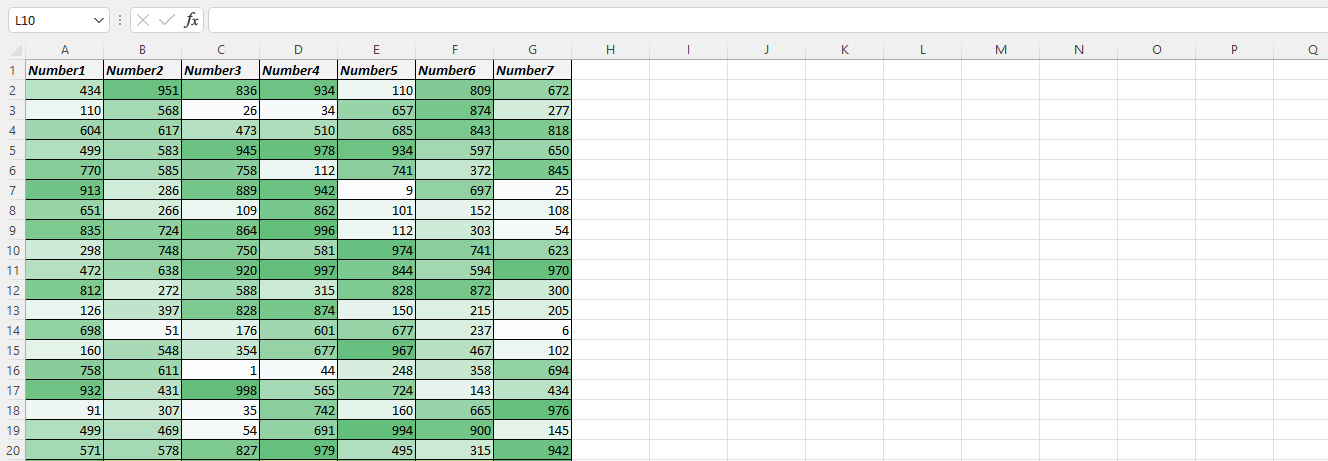
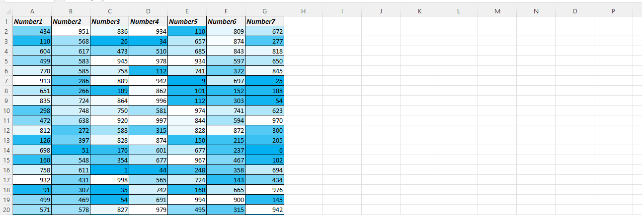
Automatically, the color scales of your range of cells indicates the ‘position‘ between the highest and lowest value.
In function of the values, the highest value is green and the lowest is white.
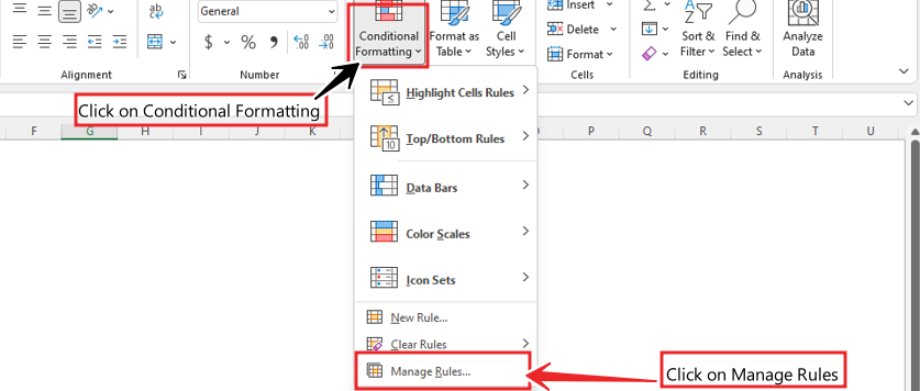
Now we will edit we will edit this cell according to us, to edit we will Select whole cell and go again to
Conditional Formatting >Manage rule>Edit Rule>Editing Format Rule

In the editing rule formatting tab, we will be able to manage the minimum value type, color and limit and maximum value type, limit and color according to us.
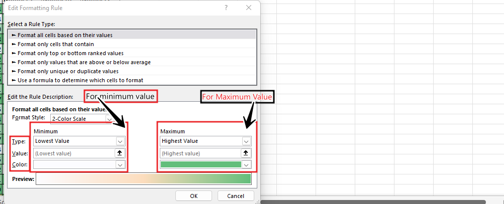
The minimum value limit is zero and the color blue and the maximum value limit is 900 and the color white is selected.
Now you can see the result.
3-Color Scale
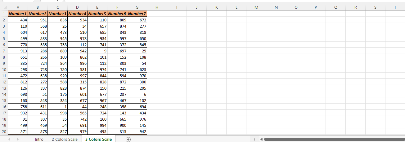
Once again we have some data in which we will be using color scales. If you look in the excel sheet you will get the data, now we will do its color formatting.
Select whole cell Activate, and click on Conditional Formatting > color_scales
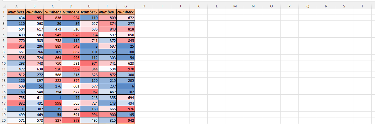
Automatically, the color scale of your range of cells indicates the ‘position’ between the highest, middle and lowest value.
In the values function, there is red for the highest value, white for the mid value, and blue for the lowest value.
Now we will edit we will edit this cell according to us, to edit we will select the whole cell and go again.
Conditional Formatting >Manage rule>Edit Rule>Editing Format Rule
In Editing Rule Formatting tab we will be able to manage minimum value type, color and limit, mid value type limit and color and maximum value type, limit and color according to our own.
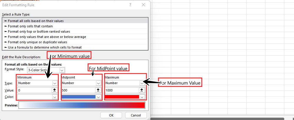
Here we have limit zero for min value and color white, 500 for mid point and color blue and max value limit is 1000 and color red is selected.
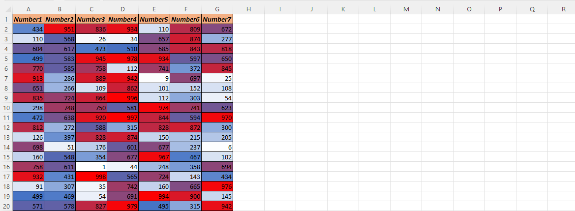
Now you can see the result.
So I hope you have understood this topic and for more information, you can follow us on Twitter, Instagram, LinkedIn, and YouTube as well.
DOWNLOAD USED EXCEL FILE FROM HERE>>
You can also see well-explained video here

