Welcome to Excel Avon
Cell Style In Excel
One of the great benefits of using preset cell styles is that if you modify the formatting associated with that style, all the cells to which that style was applied will have to go through and adjust them for you. will be updated automatically instead. Cell style is a preset format that allows you to present data visually with variations in color, cell border, alignment, and number formats.
How to Apply Cell Style in Excel
DOWNLOAD USED EXCEL FILE FROM HERE>>
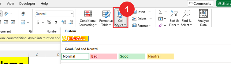
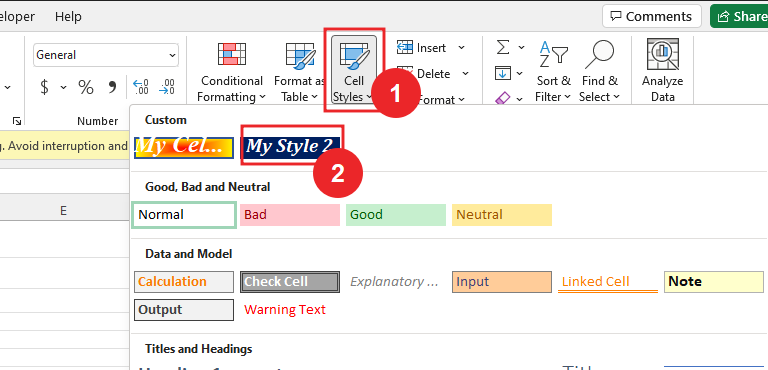
To apply or create a cell style list, you have to go to home then tap on cell style, then you will get some style made but if you want to make it according to you then you have to follow some steps on that list.
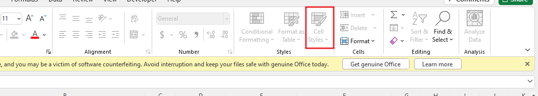
After heating the cell style, we get the cell created by Excel like this. In some versions of Excel, you’ll need to click the More dropdown button, which is an arrow with a small line at the top. In Windows systems, hovering over any of these styles will show a preview of the cell’s appearance in the active cell.
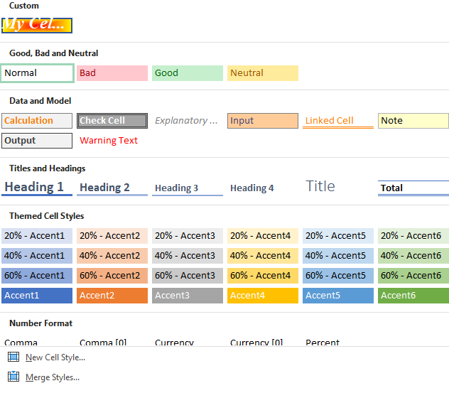
When we have to apply, we will click on any style, in that cell the style you have selected will appear. The category is given separately for the number format, which is at the bottom.
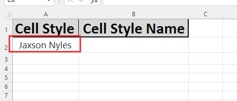
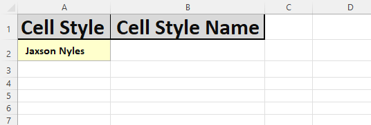
So let me show you by applying the style in an example. You can see in the given image a name is written and by selecting this cell you will go to hometab and click on cell style.
If we see many styles in cell style, then we will choose any one, we choose Note Style
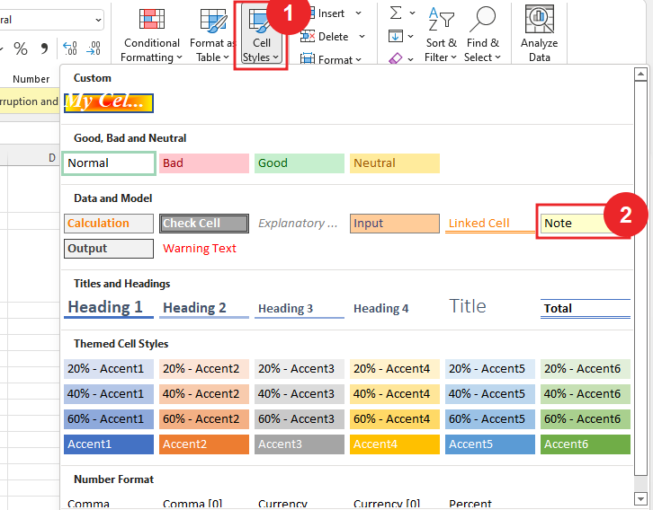
After applying note style, cell of such style is received.
How to Create a Cell Style
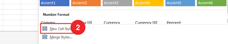
If you want to style your own cells in Excel, click New Cell Style from the Cell Styles dropdown.
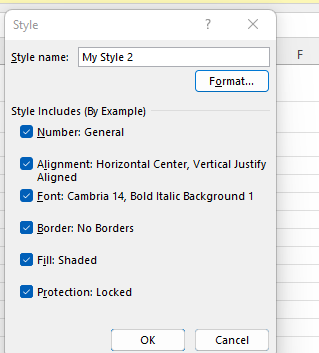
This will open the style dialog box, where you can type the name in the style name field to save your custom style with the name of your choice then go to the format option. Excel uses the format of the active cell as a starting point for your new cell style. In the example above, our new style is assumed to be an 11 point Calibri font with a normal number format. In the example above, our new style is assumed to be an 11 point Calibri font with a normal number format.
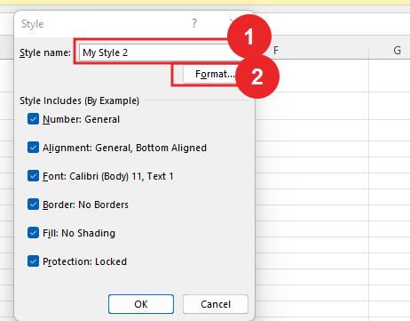
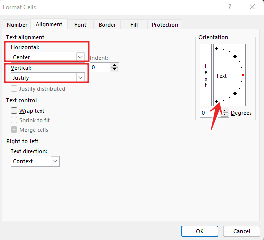
To change any attribute of the style you are creating, click the Format… button. This will open the Format Cells dialog box where you can apply and save number, alignment, font, border, fill, and protection settings. We change the alignment like we do the horizontal in the center and justify the vertical and orientation.
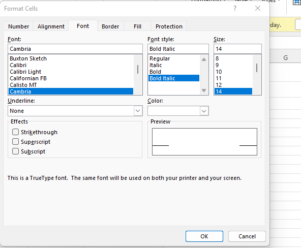
And in the format the font will be selected as Cambria, the font style will be bold italic, the font size will be 14, the font color will be white.
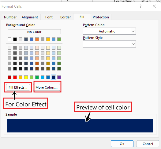
We will select the cell color in the color fill, for the cell we will select the blue color.
Now we will go to Protection option and here 2 options are available Hidden and Locked. We will do the protection locked and after locked we can not do any change in the cell
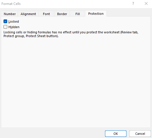
Click ok and here you can see what you did option changed. and then click ok.
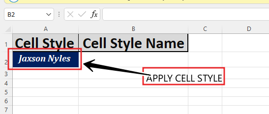
After applying, we will go to Cell style again and we will apply the cell which we have created.
By applying cell style we can see that this type of cell is found.
DOWNLOAD USED EXCEL FILE FROM HERE>>
So I hope you have understood How to Create Table Style In Excel and for more information, you can follow us on Twitter, Instagram, LinkedIn, and YouTube as well.
You can also see well-explained video here
")

")