Welcome to Excel Avon
3-D Battery Chart in Excel
DOWNLOAD USED EXCEL FILE FROM HERE>>
In today’s post we will show you how to make 3-D Battery Chart in Excel, although it is quite simple, 3-D battery chart are a great way to view information. It can easily render multiple reports with “still pending” information. Like, Remaining value, Current value, Top value, this chart can attract the viewers in seconds. Hence, using this chart can be a plus point for your professional career.
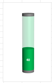
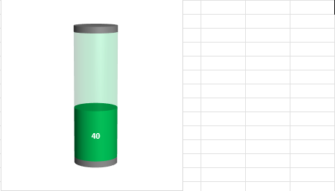
Before making a battery chart, we have to understand these things. To make a battery chart, first of all I will divide a battery into 4 parts. Bottom part, current value, remain value and Top part. I also need to divide an information into 4 parts in order to design a battery chart.
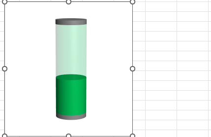
You can see how our battery chart will be made like this.
Make 3-D Battery Chart in Excel
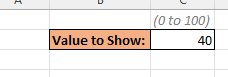
Take a cell where we will write the current value. Here the value we fill will appear in the current value part of the battery.
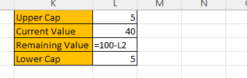
Now we will make a table here in which we will fill our values like top value, lower value, remaining value and current value of the battery. This value will be filled in the Show column for the current value and for the remaining value we will add a formula that will subtract the current value from 100.
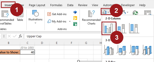
We will select the data sheet where we have written the data value. we have created go On the ‘Insert’ tab, in the Charts group, choose the Insert Column or Bar Chart button, From the Insert Column or Bar Chart dropdown list, under 2-D Bar, select Cluster Column.
Now we will change the type of chart, first click on the chart then we will go to chart design tab ‘Change Chart Type’.
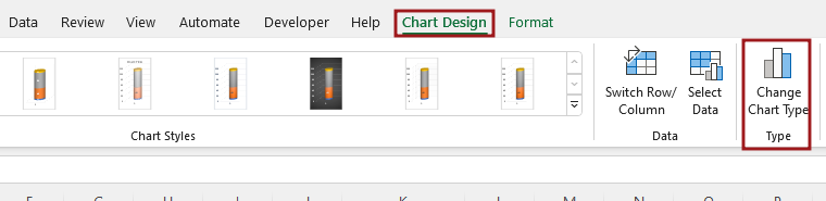
‘Change Chart Type’ will show the type of chart that we will change.
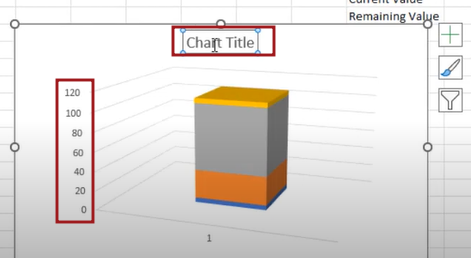
We will remove some things from the chart like title and values as well as delete the trailing walls.
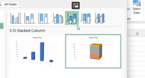
Now we will change the chart from box to cylinder type. For this, first you have to click on the chart, by clicking you will go to the data series option, by changing the battery chart, you will change it in the cylinder.

Now we will customize the battery chart, go to the Format Chart Area option and edit the X rotation and Y rotation.

The color of all parts will be according to your accord, here we will do dark gray for top, light gray for lower cap, dark green for current value, then for remaining value we will take green color only but will format the transparency of remaining part as 75%. go to data series option.
Now we will add label to the battery.
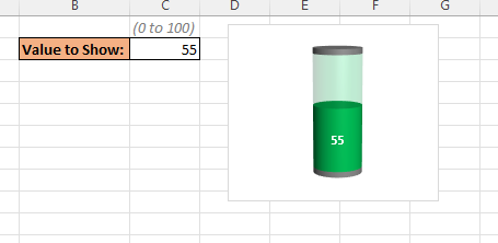
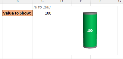
Now whatever value we write in the value show, the battery will be that much, if you repeatedly change the value of the value show cell, then the battery will be updated.
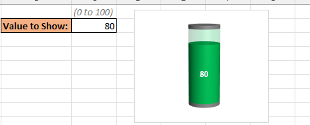
If you change the value of the cell, then the battery chart will be updated You can see the charts in the image below.
Therefore, I hope that you have understood How to make 3-D Battery Chart in Excel, maybe if you do not understand some options, then you can comment us, which we will answer soon and for more information, you can follow us on Twitter, Instagram, LinkedIn and you can also follow on YouTube.
LEARN MORE DASHBORAD AND CHART TOPIC HERE
DOWNLOAD USED EXCEL FILE FROM HERE>>
You can also see well-explained video here about How to make 3-D Battery chart in Excel.


