Welcome to Excel Avon

Basic Gantt chart in the Excel

DOWNLOAD THE USED EXCEL FILE FROM HERE>>

In today’s post we will explain how to create a Gantt chart in excel, yes it has been a bit different, Gantt charts are essential tools for project managers. But if you’re a beginner or only need this type of chart for a project, you can save money on expensive software and create a Gantt chart in Excel. A Gantt chart is a graph that shows a project schedule, its first iteration being a simple bar chart. The Gantt chart evolved into a more modern visualization for displaying not only the schedule but also the relationships and dependencies within the project schedule.

In this article, I will teach you to create basic Gantt chart in Excel step by step with pictures.

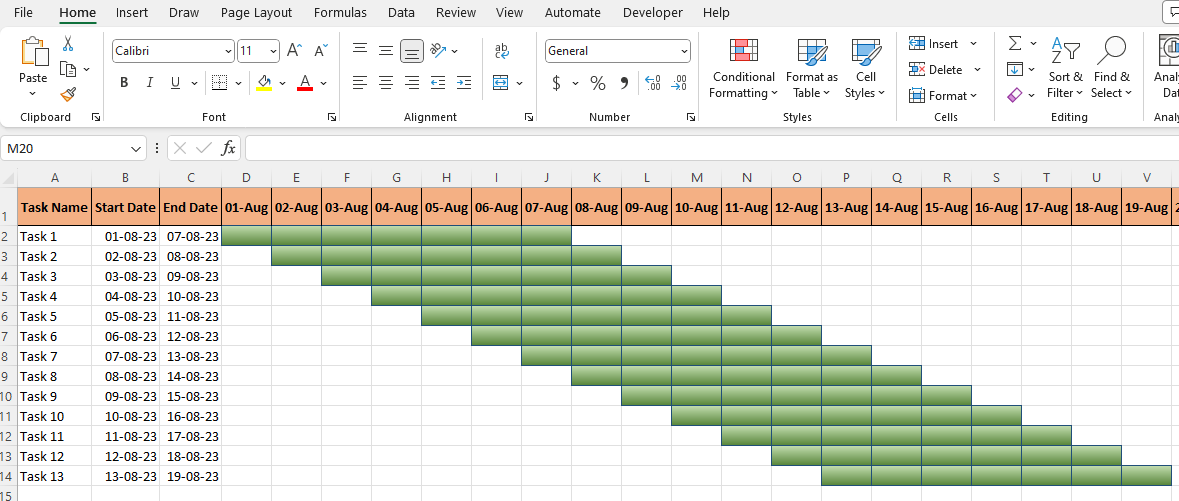
Well, as you can see, our Basic Gantt chart is going to be like this.

Prepare some data for the basic gantt chart

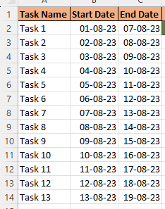
We will have some data like this and in which there will be task in one column, start date of task in second column and end date of task in third column, now we have to make a Gantt chart for this which comes in basic chart type.

Create basic gantt chart in excel

After this we will now declare the row for the month where the dates of the entire month will be. as you can see in the image below. You may not be able to see the date, but you can write the date according to your task.

How to Create a basic Gantt chart in the excel

Now select the entire range of the time period you have create for task schedule.

Make conditional formatting with dates

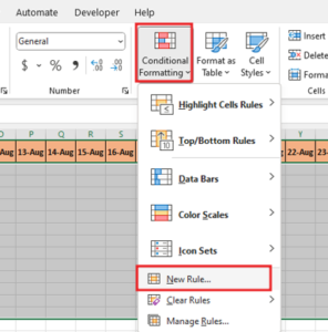
After selecting the range will go to conditional formatting. After clicking conditional formatting, we will go to new rule option.

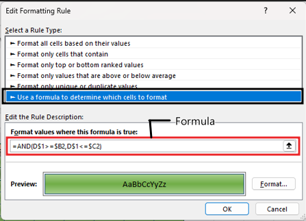
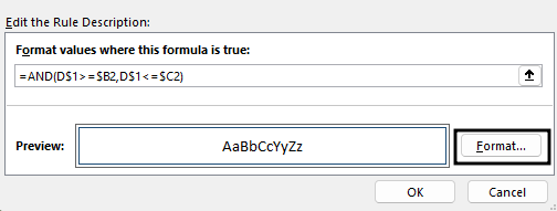
How to Create a basic Gantt chart in the excel2

After clicking in the new rule ‘Use a formula to determine which cells to format‘ will select this rule type. Now let me explain you the formula. AND Function will return the value only if all conditions are true, the first result will be for D1 but for the second result the column will have to be changed so let’s keep the row fixed. Now we will fix the start date column here, will not fix the row, copy the first condition for the second condition, then we will fix the end date column, not the row.

How to Create a basic Gantt chart in the excel4

After Select the rule type, you can format the cell by clicking on the Format button.

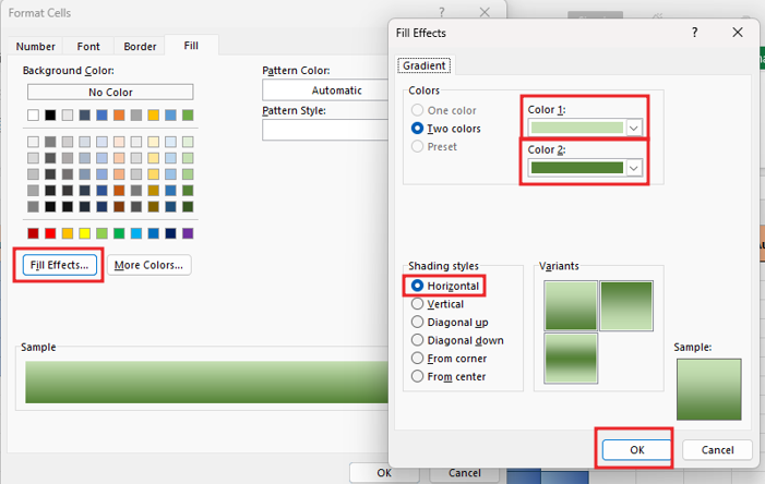
How to Create a basic Gantt chart in the excel 5

Now you can color formatting with fill effect to according to you. Here we select 2 Color And select shading styles.

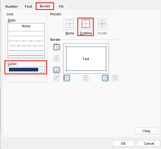
How to Create a basic Gantt chart in the excel 9

After color formatting we have to do border selection. After selecting the outline and color for the border, click oK Button

How to Create a basic Gantt chart in the excel 7

Now you can see bars will start from the start date column and go to the end date column. Similarly, all the cells are according to the end and start date.

How to Create a basic Gantt chart in the excel 10

Let’s these customizable Gantt chart graph help your project see into the future.

How to Create a basic Gantt chart in the excel 10

Now our Create a basic Gantt chart in the Excel.

- The benefits of creating a Baisc Gantt chart in Excel Store all project information in one screen: With an Excel spreadsheet, all your project information is in one location. You can simply open the spreadsheet, and voilà — you’ll see all your project tasks, deadlines, and milestones.

Therefore, I hope that you have understood How to Create a basic Gantt chart in the excel, maybe if you do not understand anything, then you can comment us with the question, which we will answer soon and for more information, you can follow us on Twitter, Instagram, LinkedIn and you can also follow on YouTube.

DOWNLOAD THE USED EXCEL FILE FROM HERE>>

LEARN MORE DASHBORAD AND CHART TOPIC HERE

You can also see well-explained video here about How to Create a basic Gantt chart in the Excel