Welcome to Excel Avon
Table Style in Excel
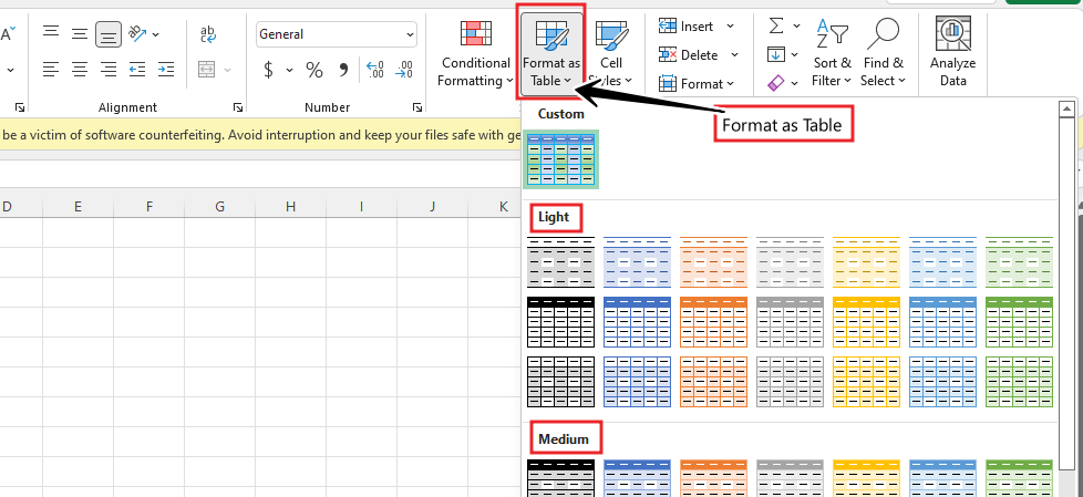
In Excel, we can see that we have been given some table styles, to apply which we can do by going to Format As Table of the Home Menu Ribbon, by accessing it, we can see that we have many table formats. where we will have 3 categories of table styles: light theme, medium theme and dark theme respectively. We can create our own customized themes for table styles, and we can clean up the table if the purpose is served.
How to Make Table Style in Excel
DOWNLOAD USED EXCEL FILE FROM HERE>>
You can also make excel table according to you, let us know how to make excel table for any random sheet. let’s see How to Make Table Style in Excel.
Steps to create Table entered in the sheet are as follows Go to Home Page>Format as Table>New Table Style

After clicking on Format As Table, we open a pop-up window like this, in which many options can be seen. ;’The first thing we need to do is to give a table name. “My Table Style.”
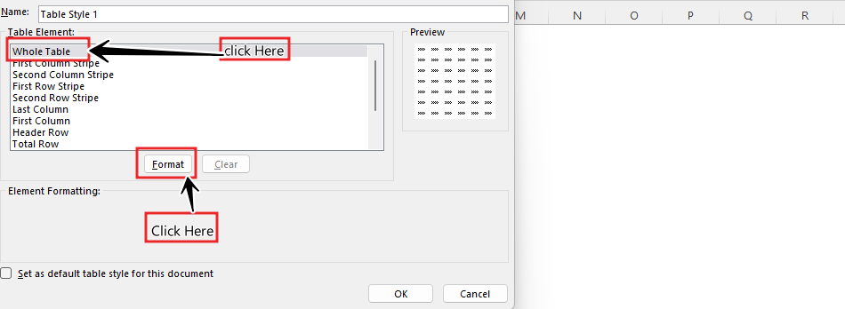
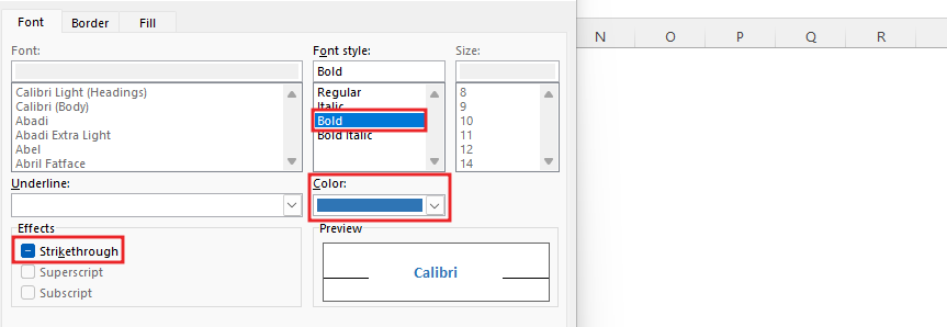
Under the “Table Element,” we must select the topic we want to modify. Firstly, we have chosen “Whole table. Then, click on format and give the formatting. For example, for “Font,” we have provided “Blue color, “Font Style,” “Bold,” and in “Underline,” “None.”
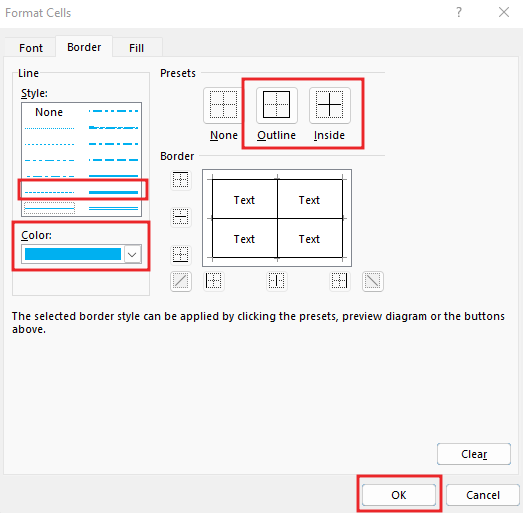
Now we will go to border option and manage accordingly. for “Border,” we have provided “blue” color, “Border Style,” “Dark,” and in “present,” “outside and inside.”
After Border, Now when I open the Fill option, you can see that you can Fill the Effect , Fill Background, Pattern Color and Pattern Style in the fill option.
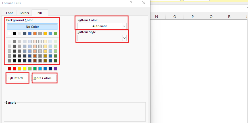
Next, we need to click “OK” to complete. Finally, we have created a style for our “whole table” and we can see the preview.
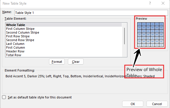
Header Row
Again Under the “Table Element,” we must select the topic we want to modify. Firstly, we have chosen “Header Row.”
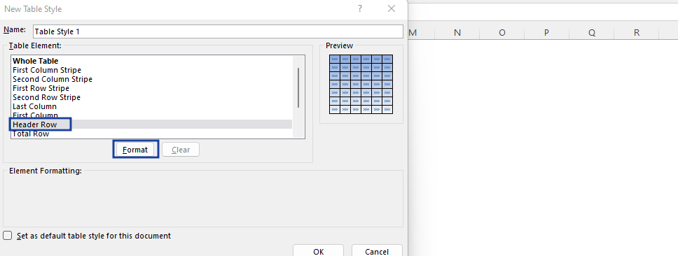
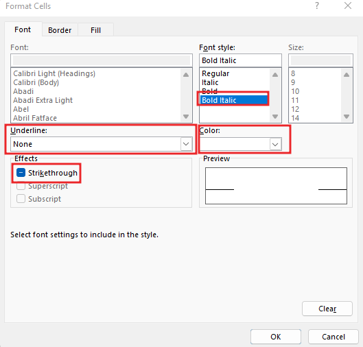
Then, click on Format in Excel and give the formatting. For example, for “Font,” we have provided “White” color, “Font Style,” “Bold Italic,” and in “Underline,” “None,” and in “‘Effect,” “Strikethrough,”.
Now, we must go to the “Fill” and select the background color.
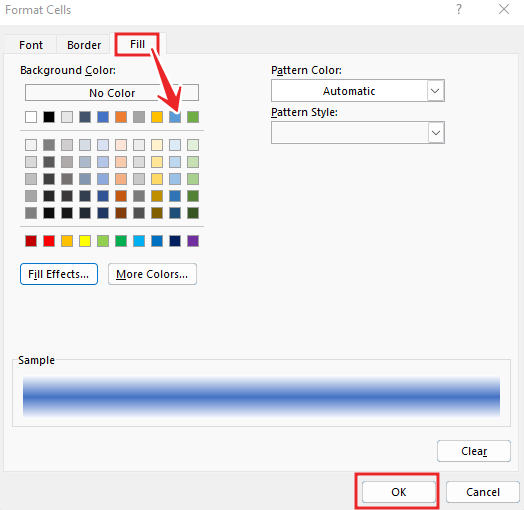
Next, we must click on “OK” to complete. Finally, we have created a style for our “Header Row,” and we can see the preview.
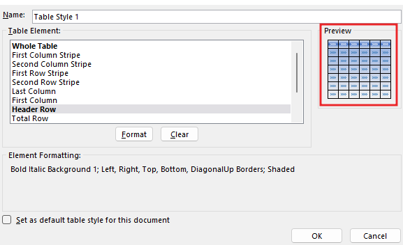
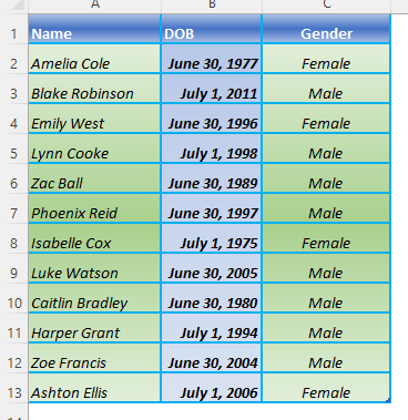
We have created our table format in Excel. Next, we must apply and see the table style in Excel. Then, under the “Design” tab, click on the drop-down list of “Table Styles.” Firstly, we may see the “Custom” table created and select that table style.

Now, we have applied our table format style in Excel.
Note:
We can play with many formulas by applying the “Total Row” option.
We must always give a table a name because it is easy to find which tables are working on.
We need to ensure that the “My data has headers” checkbox is ticked while creating a table.
DOWNLOAD USED EXCEL FILE FROM HERE>>
So I hope you have understood How to Make Table Style in Excel and for more information, you can follow us on Twitter, Instagram, LinkedIn, and YouTube as well.


