Welcome to Excel Avon
Image lookup in Excel
In this post we are talking about Image Lookup formula. To use the image lookup, we use two formulas, the first offset formula and the second match formula is used. we use these formulas to define image cell reference (a Named range) in Name manager.
OFFSET Formula
Returns a Reference to a range that is given number of rows and columns from given reference
OFFSET(reference, rows, cols, [height], [width])
MATCH Formula
Returns relative positions of an item in range or array by matching specific value in range or array.
MATCH(lookup_value, lookup_array, [match_type])
How to Use Image lookup
To use the formula, we have to go to the formula and then click in the name manager. Once the name manager is opened we will write a new name for the Image range. And then we will use offset and match formula
So now let’s move to the example and apply the formula, let’s see how it will work. As you guys can see that I have created 2 column in which one side is image and other side is name so now we will apply formula to see if this formula will work.
I will lookup Image to cell F2 Based on value in Cell E2 Matching from Range A2:A6 Range”
You can download Excel file from here>>
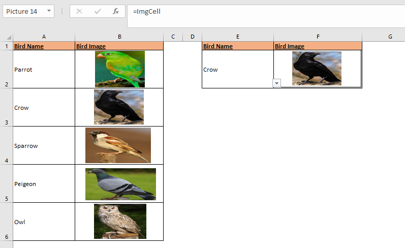
Go to Formulas tab and go to ‘Name Manager’ Option to define an image reference cell (dynamic cell) based on offset and match formula

Once the name manager is opened we will write a new name for the Image range
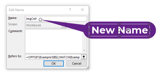
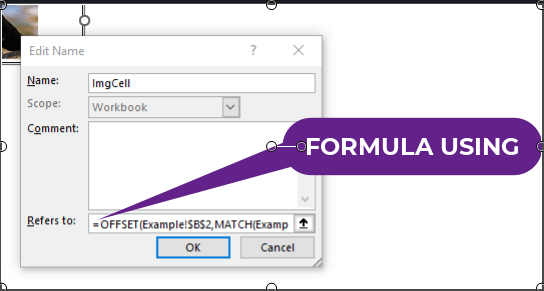
=OFFSET(Example!$B$2,MATCH(Example!$E$2,Example!$A$2:$A$6,0)-1,0)
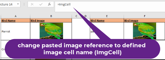
After writing the formula, we will copy the first cell(B2) of the image range and paste it in cell F2 as linked image.
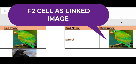
Now I will change pasted image reference to defined image cell name (ImgCell)
You can download used Excel file from here>>>
Now you can try change lookup image value. So I hope you have understood this formula and for more information you can follow us on Twitter, Instagram, LinkedIn and YouTube as well.
You can also see well explained video here


