Welcome to Excel Avon
3-D Progress circle chart in Excel
DOWNLOAD USED EXCEL FILE FROM HERE>>
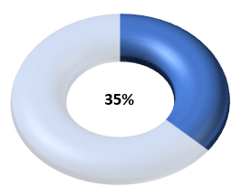
Create 3-D Progress circle chart in Excel
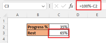
Create a table in excel sheet which will look something like this. In which there will be 2 Values. Progress and Left Progress. Added formula for Left Progress =100%-C2.
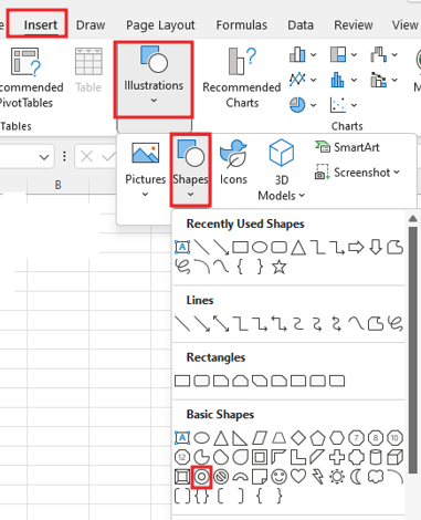
Without selecting any data, insert a circle Hollow shape by going to insert tab> Illustrations> Shapes> Basic Shape > Select Circle Hollow.
Drag the select shape in the sheet, yes many of you will think this is a doughnut chart which is not really it is a shape which looks like a doughnut chart.
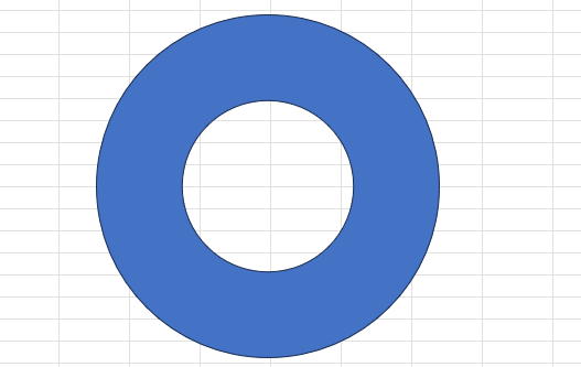
After drawing this chart, you can fix the shape manually from Size option.

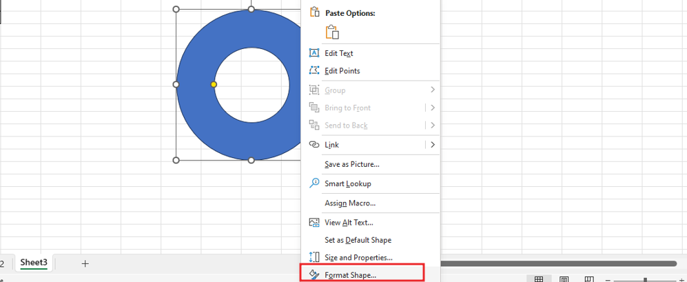
Right click on the chart then go to Format shape option.
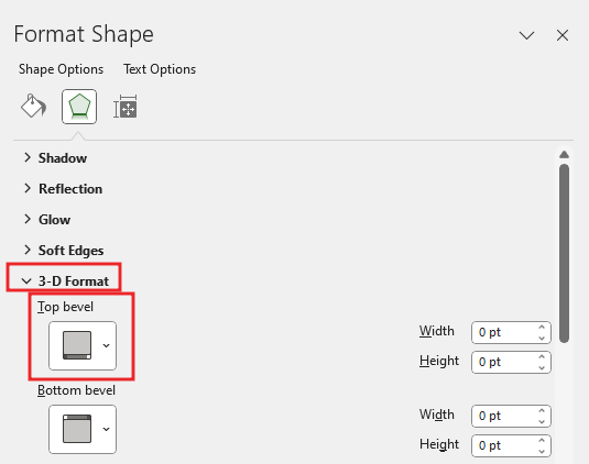
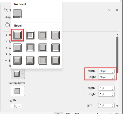
Now you have to do 3-D formatting of this shape. Go to 3-D format option and make the top bevel soft rounded. Increase the amount of width and height of the effect 3-D Effect.
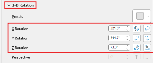
Now you have to do 3-D rotation, go to the 3-D rotation of the shape, then rotate the X rotation or rotation and Z rotation according to your accordion, you can see as the value is written below.
Now our chart looks something like this
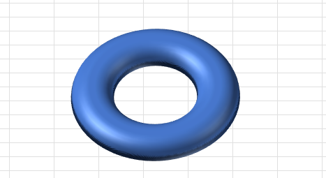
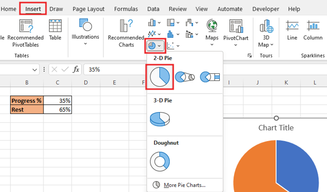
Now we will insert 2-D Pie Chart by going to Insert tab. with selecting data.
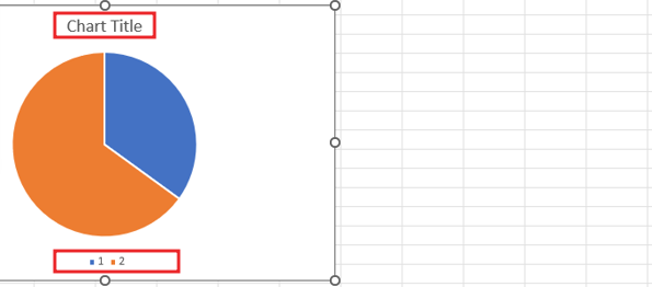
Now Delete the legend and chart title from the chart.
Now you No Fill the background of chart also remove outline from the chart.
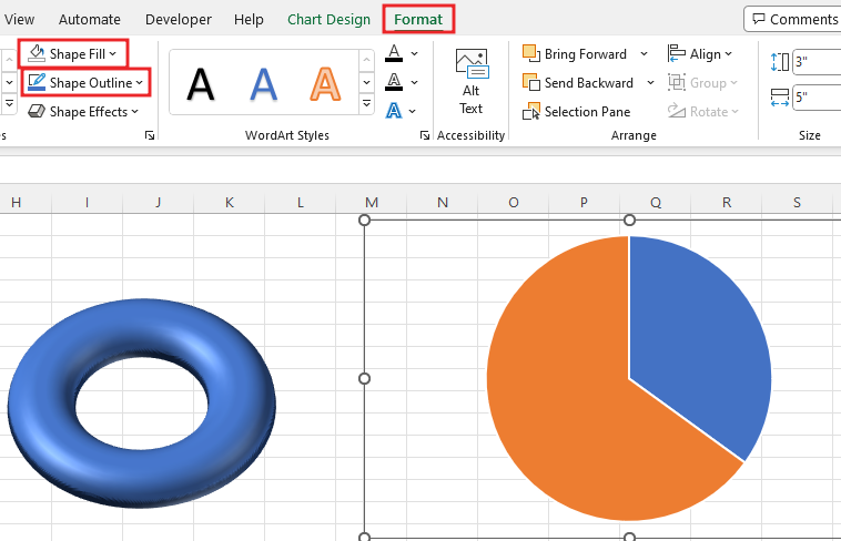
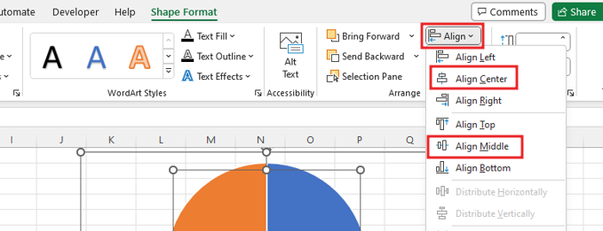
Now select both the shape and the chart, then align it.
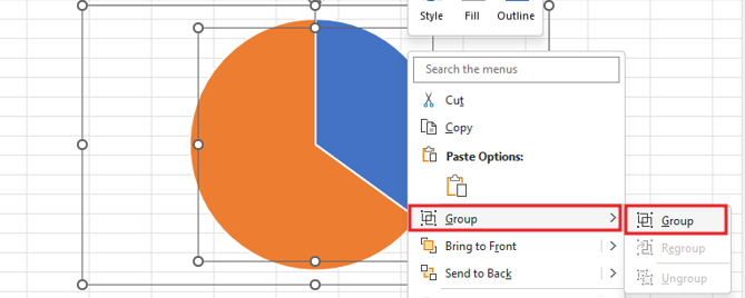
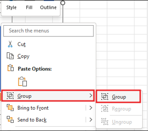
Select the shape and chart and group them.
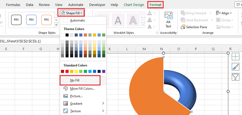
Now Select the blue part and go to the format tab. And No Fill for the blue part with No outline.
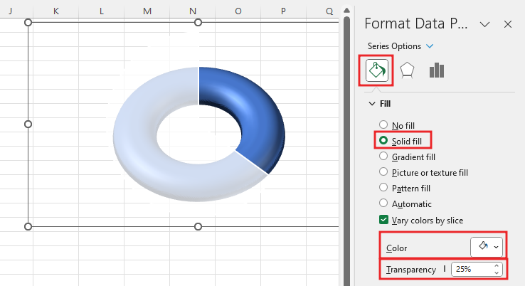
Now select the orange part and go to the format option and fill it solid and then fill this part with white color and make its transparency 25%.
Go to insert tab and select it in the text box and drag it Center of the chart. remove the background and outline of the text box by going to the Format option with No Fill and No Outline.
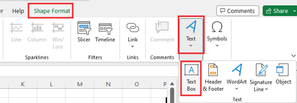
Add formula in Text Box =C2. after aligning the text box. Customize text box, Bold, size of font color, size of font.
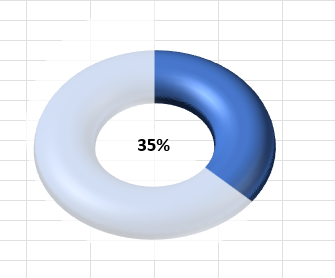
Select the shape and Textbox then group both.
Go to view tab and remove gridline from chart.
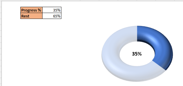
Now our 3-D progress Circle Chart in Excel. change the value of cell then you can see chart has been changed.
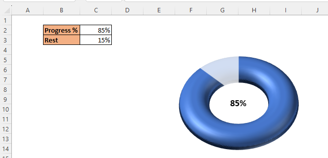
Therefore, I hope that you have understood How to Create 3-D progress Circle Chart in Excel, maybe if you do not understand anything, then you can comment us with the question, which we will answer soon and for more information, you can follow us on Twitter, Instagram, LinkedIn and you can also follow on YouTube.
DOWNLOAD USED EXCEL FILE FROM HERE>>
LEARN MORE DASHBORAD AND CHART TOPIC HERE
You can also see well-explained video here about How to Create 3-D progress Circle Chart in Excel


