Welcome to Excel Avon
Circle Progress Chart in Excel
DOWNLOAD THE USED EXCEL FILE FROM HERE>>
In today’s post we will show you how to create circle progress chart in excel, although it is quite simple, A circle progress chart is a graph that displays the progress made toward a certain goal. We’ll use special formatting tricks in Excel to create the circle progress chart. This Excel progress chart will come with a fully updatable graph. Modern Excel charts and templates are easy to build using built-in shapes, icons, and other custom formatting tricks to grab your audience’s attention.
We love this chart type because they allow us to track and display the progress of a single performance indicator. Generally, we can create a progress circle chart by simply inserting a doughnut chart. But, this chart can be unattractive and vague sometimes as default. Regarding this, with some customizations, we can create an excellent-looking progress circle chart in Excel.
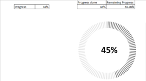
You can see how our circle progress chart will be made like this.

Create Circle Progress Chart in Excel
Take a cell where we will write the progress to be displayed in the chart and create another table where progress done and remaining progress will be shown.

The formula will be applied in the complete progress cell, the value that is in c2 will be filled in the same complete progress cell (=C2).

Subtract completed progress cells from 100 for remaining progress value.

Now we will take blank cell where we will use REPT function and write “1,” 100. repeat text the given no. of times. Delete last comma and copy all text.


Go to the ribbon, locate the insert tab and select a doughnut chart.
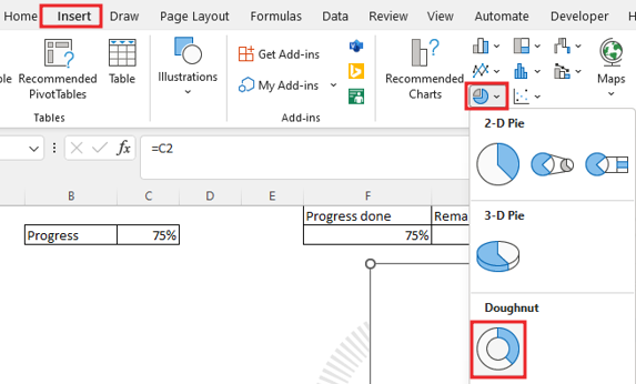
Now we will right click on the chart then click on option in select data and where we will add series name and add data here, we will paste the text which was found by REPT function. we will click the OK button

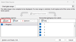

Go to the elements of the chart, then remove the title, legend from here.

Now we will do the color formatting of the chart by clicking on the chart, color solid gray, solid border white color and border width 2.25pt.
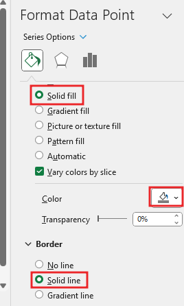
Again, we will go to the chart and then again in the chart we will go to the select data option.

Now add legend entries. we will write the series name, in the series value, we will add cell from F2 To G2.
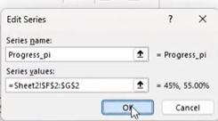
Our chart is starting to look something like this.
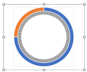
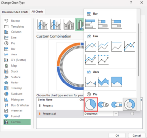
Now we will click on the later chart. then go to chart design tab click on change chart type. here we will add the pie chart.
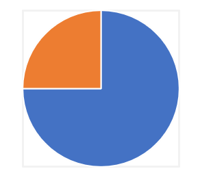
Blue part is complete progress. and orange part is remaining.
By clicking on the blue part, you will have to go to format Data point. Now we’ll Color formatting on chart.
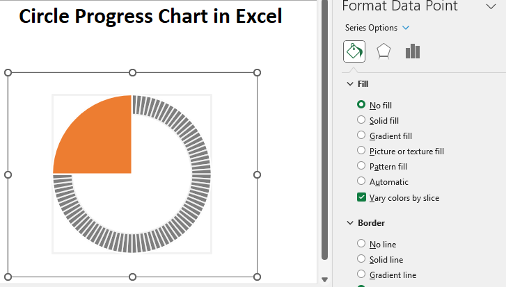
Also, change the color of the remaining orange part to white by going to color formatting. Keep the color of the remaining part as transparency 20%.
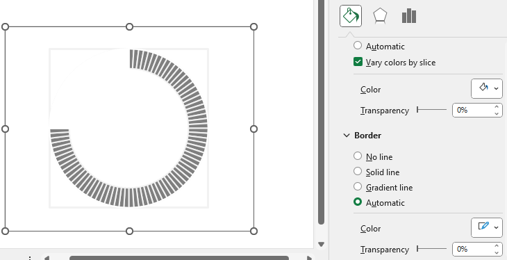
Now we will add text box to the chart. Add formula in the text box =C2.

As our chart is ready, if we update the chart, then the progress of the chart will keep changing.
Therefore, I hope that you have understood How to Create Circle Progress Chart in Excel, maybe if you do not understand anything, then you can comment us with the question, which we will answer soon and for more information, you can follow us on Twitter, Instagram, LinkedIn and you can also follow on YouTube.
DOWNLOAD THE USED EXCEL FILE FROM HERE>>
LEARN MORE DASHBORAD AND CHART TOPIC HERE
You can also see well-explained video here about How to Create Circle Progress Chart in Excel


