Welcome back to Excel Avon
How to use COUNTIFS formula in Excel
Summary
The COUNTIFS excel function counts the values of the supplied range based on one or multiple criteria or conditions. The supplied range can be single or multiple and adjacent or non-adjacent. Being a statistical function of Excel.
Formula
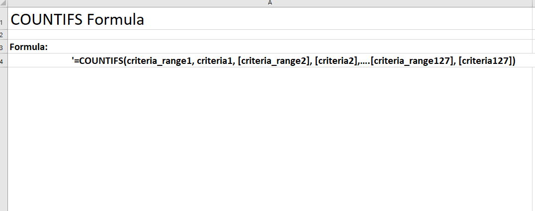
=COUNTIFS(RANGE1,CRITERIA1,[RANGE2],[CRITERIA2],…………………….)
Argument–
RANGE1- This is the first range within which value are to be counted.
CRITERIA1- The criteria1 is use on RANGE1
RANGE2- This is the second range within which value are to be counted.
CRITERIA2-Optional. It is used to determine which cells to count criteria2 is applied against range2.
Result- The COUNTIFS formula return numeric value.
NOTE–
-
-
Non-numeric criteria needs to be enclosed in double quotes but numeric criteria does not.
 For example: "50", "70", ">80", "LIMIT", or A1 (where A1 contains a number).
-
 In case of multiple range and criteria pairs, the COUNTIFS counts only those cells that
 meet all the specified conditions.
-
Multiple conditions are applied with AND logic, i.e. condition 1 AND condition 2, etc.
How to use COUNTIFS formula in Excel
-
Example-1
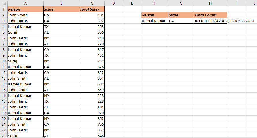
In first example I will show you how to use COUNTIFS Formula. I had made person per state and total sales I will get the total count of person per state, so I will use here COUNTIFS formula so I will use here-
=COUNTIFS(A2:A38,F3,B2:B38,G3) and press enter. Now this getting the total.
Where- A2:A38 Is the first range
F3 is the Criteria1
B2:B38 is the second range
G3 is second range
(according attached below image)
Example-2
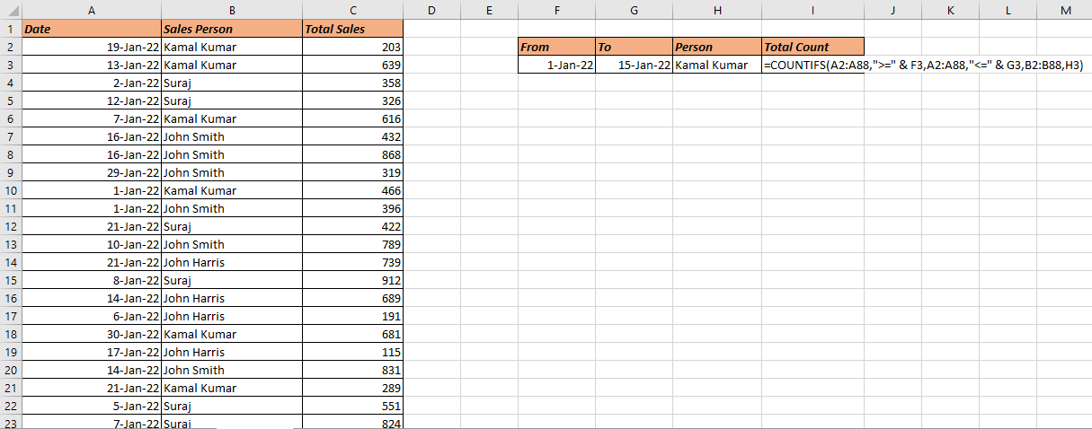
In second example I have made a data, based on state sales person & total sales, I want to calculate the Occurance of KAMAL KUMAR has how many time search b/w two date I will write =COUNTIFS(CRITERIA1,RANGE1,[CRITERIA2],[RANGE2],…………..) and I make the first criteria write here-
=COUNTIFS(A2:A88,”>=” & F3,A2:A88,”<=” & G3,B2:B88,H3) and press enter.
A2:A88 is the Range1
“>=” & F3 is the criteria
“<= & G3 is the second criteria
B2:B88 is Range2.
H3 is criteria.
(according attached below image)
You can also see well explained video here


")